1. Wave propagation in solid medium in time
UMR Géosciences Azur – CNRS – IRD – UPMC - UNSA
Wave propagation in solid medium in time
By J. Virieux and S. Operto
Ecole thématique CNRS-CGG-UNSA SEISCOPE
11-15 septembre 2006

2. Acknowledgments
Victor Cruz-Atienza (Géosciences Azur on leave for SDSU) FDTD
Matthieu Delost (Géosciences Azur on leave) Wavelet tomography
Céline Gélis (Géosciences Azur now at Amadeous) Full wave elastic imaging
Bernhard Hustedt (Géosciences Azur now at Shell) Wavelet decomposition of PDE
Stéphane Operto (Géosciences Azur/ CNRS CR) full researcher
Céline Ravaut (Géosciences Azur now at Dublin) Full acoustic inversion
Spice group in Europe :
FDTD introduction :
ftp://ftp.seismology.sk/pub/papers/FDM-Intro-SPICE.pdf
By P. Moczo, J. Kristek and L. Halada

3. Non-Translucid Earth 1
Inside the Earth, discontinuities are present which lead to converted phases, especially in the crust : three characteristic times in seismograms/traces
We need techniques for modelling these waves which can be quite complex

4. Anatomy of seismic waves phases
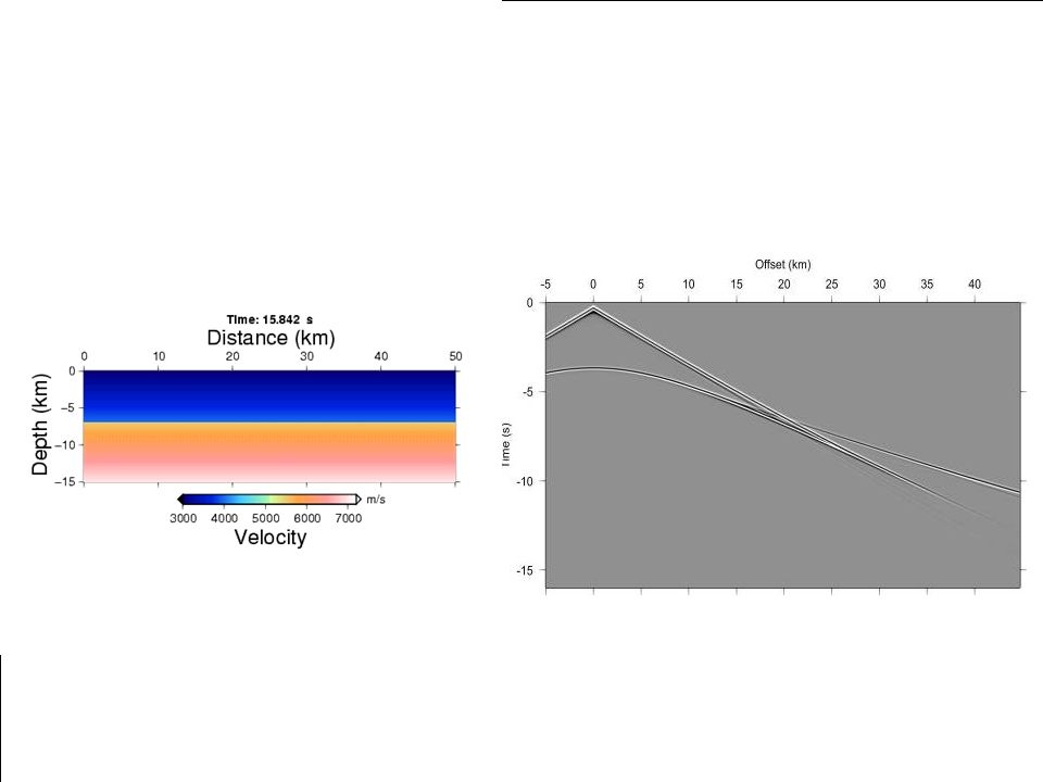
ANATOMY OF GLOBAL-OFFSET DATA
From Stéphane Operto
Velocity gradient at interfaces : diving waves

5. Anatomy of global-offset seismograms:
Continuous sampling of apertures from transmission to reflection

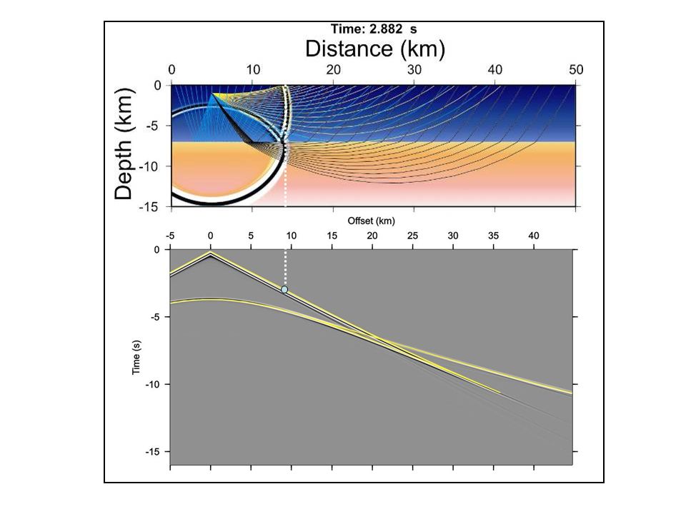
9. Critical incidence – total reflection

11. Upgoing conic wave

12. Critical distance

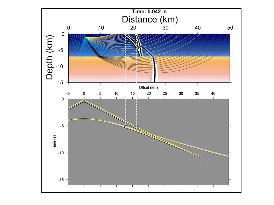
15. Conic wave
Interface wave

17. Root wave

18. Asymptotic « convergence » between direct and super-critical reflected waves

19. Diving wave

20. Synthetic seismograms
Diving Wave
Head or conic wave

22. LA PROPAGATION DES ONDES I
Tenseur de contrainte exprime les forces internes (séismes)
Tenseur de déformation
à partir du déplacement
en présence de forces
Le PFD
La loi de Hooke
avec les coeffs. élastiques
L’équation
est dite
l’équation de l’élastodynamique
Une rhéologie simple pour des milieux LHI
en fonction des coefficients de Lamé !

23. LA PROPAGATION DES ONDES II
L’équation élastodynamique en milieu linéaire et élastique
en milieu linéaire, élastique. C’est un système de 3 équations du second ordre aux dérivées partielles définissant les composantes ui(x,t). Un système à 9 équations peut aussi être construit à partir des vitesses et des contraintes :
où la fonction mij est non nulle dans les régions sources.

24. LA PROPAGATION DES ONDES III
L’équation élastodynamique en milieu linéaire, élastique et isotrope s’écrit
On utilisera fi ou fi - mij suivant les besoins. On parlera de systèmes de forces équivalents.

25. LA PROPAGATION DES ONDES IV
Dans des milieux liquides, on préfère travailler avec la pression et la vitesse des particules
On en déduit les équations d’onde acoustique
où la fonction q(x,t) s’appelle la source volumique en vitesse et est définie par

26. LA PROPAGATION DES ONDES V
Si on élimine la vitesse des particules, on obtient l’équation d’onde acoustique scalaire pour la pression p(x,t) :
avec
Si on suppose que la masse volumique est homogène, on a
avec
qui est l’équation d’onde scalaire que l’on retrouve dans différents livres

27. LA PROPAGATION DES ONDES VI
Si on élimine la pression, on obtient l’équation d’onde acoustique vectorielle
avec la force en vitesse suivante
Cette équation est un cas particulier de l’équation dérivée de l’équation élastodynamique. En général, on ne l’étudie pas séparément et on ne considère que l’équation d’onde acoustique scalaire.

28. Considérons l’équation d’onde scalaire
Si les termes sont nuls, alors l’excitation peut se déduire d’un terme excitation en divergence :
que nous pouvons mettre sous une forme vectorielle

29. LES FONCTIONS DE GREEN
La réponse impulsionnelle définit la fonction de Green G(x,t;x0,t0) du milieu où la source ponctuelle se trouve en x0 et l’impulsion est donnée en t0,.tandis que l’on calcule la solution au point x et au temps t.
où c(x) est la vitesse et la distribution dirac est notée par d
et peut se voir comme une fonction de valeur infinie en zéro.

30. Les solutions en milieu homogène
Solution 1D
Solution 2D
Solution 3D
Certaines caractéristiques communes mais d’autres très différentes comme la trainée à 2D

31. The corner-edge as a complex example

32. ODE versus PDE formulations
Non-linear
Linear
O.D.E
Ordinary differential Equations
P.D.E
Partial Differential Equations
GOAL : find ways to transform differential operators into algebraic operators in order to use linear algebra at the end
Symmetry between space and time ?

33. An apparent easy way
Spectral methods allow to go directly to this algebraic structure
Dispersion relation has to be verified BUT conditions have to be expressed in this dual space : here is the difficulty !
Pseudo-spectral approach : a remedy for a precise and fast strategy
Go to the dual space only for computing spatial derivatives and goes back to the standard space for equations and conditions
Frequency approach of Pratt : the opposite way around

34. 3D Elasto-dynamic equations
Divide by the density will leave medium properties only on the RHS
The previous PDE form is then retrieved

35. P-SV equations Elastic properties No attenuation
Medium properties vary from point to point
No spatial derivatives of these medium properties

36. One-dimensional scalar wave
The scalar wave equation is verified by the vibration u(t,x)
Homogeneous medium
The wave solution is u(x,t)=F(x+ct)+G(x-ct) whatever are F and G (to be checked)
The wave is defined by pulsation w, wavelength l, wavenumber k and frequency f and period T. We have the following relations
A plane wave is defined by
with the dispersion relation
The phase velocity is for any frequency
If the pulsation w depends on k, we have
and the group velocity is
which is identical to phase velocity for non-dispersive waves

37. First-order hyperbolic equation
stress
Let us define other variables for reducing the derivative order in both time and space
The 2nd order PDE became a 1st order PDE
velocity
This is true for any order differential equations: by introducing additionnal variables, one can reduce the level of differentiation. Among these different systems, one has a physical meaning
which becomes
with
Other choices are possible as displacement-stres instead of velocity-stress.

38. Characteristic variables
Consider an linear system is defined by
If the matrix A could be diagonalizable with real eigenvalues, the system is hyperbolic.If eigenvalues are positive, the system is strictly hyperbolic.
The system could be solved for each component fp
The curve x0+lp t is the p-characteristic
The scalar wave introduces w=(v,s) and the following matrix w(u,d) where u design the upper solution and d the downgoing solution.
The transformation from w to f splits left and right propagating waves

39. Other PDE in physics
The scalar wave equation is a partial differential equation which belongs to second-order hyperbolic system.
Wave Equation
Fluid Equation
Diffusion Equation
Laplace Equation
Fractional derivative Equation
Time is involved in all physical processes except for the Laplace equation related to Newton law and mass distribution.
Poisson equation could be considered as well when mass is distributed inside the investigated volume
Poisson Equation

40. Initial and boundary conditions
Initial conditions u(x,0)
1D string medium
Boundary conditions u(0,t)
Boundary conditions u(L,t)
Dirichlet conditions on u
Neumann conditions on s
f(x,t) Excitation condition
Difficult to see how to discretize the velocity !
Much better for handling heterogeneity

41. Finite Difference Stencil
Truncations errors :
(Leveque 1992)
Higher-order terms : same procedure but you need more and more points
Second derivative

42. Discretisation and Taylor expansion
Assuming an uniform discretisation Dx,Dt on the string, we consider interpolation upto power 4
by summing, we cancel out odd terms
neglecting power 4 terms of the discretisation steps. We are left with quadratic interpolations, although cubic terms cancel out for precision.

43. Other expansions
ei(x) could be any basis describing our solution model and for which we can compute easily and accurately either analytical or numerical compute derivatives
A polynomial expansion is possible and coefficients of the polynome could be estimated from discrete values of u: linear interpolation, spline interpolation, sine functions, chebyshev polynomes etc
Choice between efficiency and accuracy (depends on the problem and boundary conditions essentially)

44. Consistency Local error Taylor expansion around (ih,mDt)
FD scheme is consistent with the differential equations (do the same for the other equation)

45. Stability Harmonic analysis in space and in time
w is complex : the solution grows exponentially with time : UNSTABLE
Local stability # long-term stability (finite domain validity)
CONSISTENCE + STABILITY = CONVERGENCE (not always to the physical solution)

46. STABLE STENCIL :leap-frog integration
m+1 m
m-1
i i i+1
Harmonic analysis
is real
The solution does not grow with time : STABLE
CFL condition
Courant, Friedrichs & Levy
Magic step Dt=h/c0
Characteristic line
The time step cannot be larger than the time necessary for propagating over h
Von Neuman stability study

47. Time integration (more theory)
Euler
Backward Euler
Left-side (upwind)
Right-side
Lax-Friedrichs
Leapfrog
Lax-Wendroff
Beam-Warming

48. UNCOUPLED SUBGRID : SAVE MEMORY
RED-BLACK PATTERN
i-1 i
i+1
m-1 m
m+1
The staggered grid
UNCOUPLED SUBGRID : SAVE MEMORY
ONLY BOUNDARY CONDITIONS WOULD HAVE COUPLED THEM
STAGGERED GRID SCHEME
INDICE FORTRAN ?
Second-order in time & in space

49. NUMERICAL DISPERSION Moczo et al (2004)
How small should be h compared to the wavelength to be propagated ?
2ème ordre
4ème ordre

50. NUMERICAL ANISOTROPY
PSG
FSG
COMBINE ?

51. PARSIMONIOUS RULE
How to define these discrete values for an heterogeneous medium ?
(especially when considering strong discontinuities)
How to estimate the spatial operator
Do same thing for r

52. FREE SURFACE (Neumann condition)1 2
m-1 m
m+1
Amplitude deficit of wave nearby the free surface 1 2
m-1 m
m+1
We can see that we have amplified by a factor of 2
Antisymmetric stress

53. ESIM procedure SAT procedure 1 2 m-1 m m+11 2
m-1 m
m+1
Predict by extrapolation values outside the domain for keeping the finite difference stencil while verifying solutions on the boundary
SAT procedure
Modify the stencil when hitting the boundary for keeping same accuracy while using only values on one-side of the boundary
SAT has a mathematical background while ESIM has not

54. Source or grid excitation
Impulsive source
The source is a term which should be added to the equation. Because it is related to acceleration, we denote it as an impulsive excitation.
Known solution
A particular solution of the wave equation is injected into the medium or the grid. Typically an incident plane wave is applied at each grid point along a given line.
Explosive source
A very popular excitation is the explosive source, which requires either applications of opposite sign forces on two nodes or a fictious force between two nodes. Once integration has been performed, we should add

55. Radiative boundaries
One may assign boundary conditions as if the medium was infinite, also known as radiative conditions. These conditions may be very complex to design if the medium is heterogeneous.
For the 1D case, we may simply say that
which again is exactly verified for the magic step of characteristics. For other time steps, interpolation between t-Dt and t-2Dt.
In 2D and 3D, the shape of the wavefront must be introduced in an attempt for absorbing waves along boundaries and we shall see that other techniques rather radiative conditions may be considered (p-characteristics).
The Perfeclty Matched Layer concept turns out to be very efficient (Berenger, 1994).

56. ABC : PML conditions
On conserve des variables à intégrer qui suivent la propagation dans une direction

57. Energy balance
PML absorption is better than absorption by other methods at any angle of incidence (at the expense of a cost in time domain)

59. 3D test of PML conditions
Left : finite box with Neuman conditions
Middle : PML
Right : difference between true solution and PML solution

60. STAGGERED GRID : A FATALITY
1D : Yes (for the moment!)
2D & 3D : No (one may use the spatial extension!) X
Trick Z
3D case
FSG
PSG
Combine ?

61. Saenger stencil New staggered grid sxx,szz sxz vz vx
Local coupling between x and z directions: new staggered grid and velocity components define at a single node (as for the stress). Expected better behaviour for the interaction with the free surface (it has been verified).

62. FSG versus PSG
PSG should be preferred when one needs all components at a single node (anisotropy, plasto-elastic formulation …)

63. NUMERICAL ANISOTROPY
PSG
FSG
COMBINE ?

64. All you need is there
We have all ingredients for resolving partial differential equations in the FDTD domain.
Loop over time k = 1,n_max t=(k-1)*dt
Loop over stress field i=1,i_max x=(i-1)*dx
compute stress field from velocity field: apply stress boundary conditions; end
Loop over velocity field i=1,i_max x=(i-1)*dx
compute velocity field from stress field: apply velocity boundary conditions; end
Set external sources effects
compute by replacing OR by adding external values at specific points. If we replace, the input should be a solution of the wave equation.
End loop over time
Exercice : write the same organigram in the frequency domain.
Exercice : write a fortran program to solve the 1D equation (should be done in a WE).

65. COLLOCATION
FD method : discrete equations exact at nodes (strong formulations)
FE method : equations verified on the average over an element (to be defined with respect to nodes) (weak formulation)
FV method : equations verified on the average over an volume (only flux between volumes)

66. COLLOCATION FD dirac cumb FE method : elements share nodes !
FV method : elements share edges !
FV method requires simpler meshing as well as simpler message communications …. Usually this is the standard extension of FD modeling in mechanics

67. Finite volume method
Pseudo-flux conservative form

68. Finite volume method

69. CONCLUSION Efficient numerical methods for propagating seismic waves
Time integration versus frequency integration
Competition between FE & FV for modelling
FD an efficient tool for imaging

70. Propagation sismique dans la baie des anges
Seisme de magnitude 4.9 à 8 km de profondeur

71. THANKS YOU !