Download presentation
Presentation is loading. Please wait.

1
Softrare Reliability Methods
Prof. Doron A. Peled Bar Ilan University, Israel And Univeristy of warwick, UK Version 2008

2
Some related books: Mainly: Also:

3
Goal: software reliability
Use software engineering methodologies to develop the code. Use formal methods during code development 2

4
What are formal methods?
Techniques for analyzing systems, based on some mathematics. This does not mean that the user must be a mathematician. Some of the work is done in an informal way, due to complexity.

5
Examples for FM Deductive verification: Using some logical formalism, prove formally that the software satisfies its specification. Model checking: Use some software to automatically check that the software satisfies its specification. Testing: Check executions of the software according to some coverage scheme.

6
Typical situation: Boss: Mark, I want that the new internet marketing software will be flawless. OK? Mark: Hmmm. Well, ..., Aham, Oh! Ah??? Where do I start? Bob: I have just the solution for you. It would solve everything.

7
Some concerns Which technique? Which tool? Which experts?
What limitations? What methodology? At which points? How expensive? How many people? Needed expertise. Kind of training. Size limitations. Exhaustiveness. Reliability. Expressiveness. Support.

8
Badmouth Formal methods can only be used by mathematicians.
The verification process is itself prone to errors, so why bother? Using formal methods will slow down the project.

9
Some answers... Formal methods can only be used by mathematicians.
Wrong. They are based on some math but the user should not care. The verification process is itself prone to errors, so why bother? We opt to reduce the errors, not eliminate them. Using formal methods will slow down the project. Maybe it will speed it up, once errors are found earlier.

10
Some exaggerations Automatic verification can always find errors.
Deductive verification can show that the software is completely safe. Testing is the only industrial practical method.

11
Our approach Learn several methods (deductive verification, model checking, testing process algebra). Learn advantages and limitations, in order to choose the right methods and tools. Learn how to combine existing methods.

12
Emphasis The process: Selecting the tools, Modeling, Verification, Locating errors. Use of tools: Hands on. PVS, SPIN Visual notation: Statecharts, MSCs, UML.

13
Some emphasis The process of selecting and using formal methods.
The appropriate notation. In particular, visual notation. Hands-on experience with tools.

14
The unbearable easiness of grading
During class, choose some small project in groups, e.g., Explore some examples using tools. Implementing a simple algorithm. Dealing with new material. or covering advanced subject. - Office presentation (1 hour). - Written description (2-3 pages + computer output or 6-10 pages). - Class presentation ( hours per group).
. - Written description (2-3 pages + computer output or 6-10 pages). - Class presentation ( hours per group).")
15
Example topics Project: Advanced topics:
Verify some example using some tools. Communication protocols. Mutual exclusion. Advanced topics: Abstractions. Reductions. Partitions. Static analysis. Verifying pushdown automata. Verifying security protocols.

16
Where do we start? Boss: Mark, can you verify this for me?
Mark: OK, first I have to ...

17
Things to do Check the kind of software to analyze.
Choose methods and tools. Express system properties. Model the software. Apply methods. Obtain verification results. Analyze results. Identify errors. Suggest correction.

18
Different types of software
Sequential. Concurrent. Distributed. Reactive. Protocols. Abstract algorithms. Finite state.

19
Specification: Informal, textual, visual
The value of x will be between 1 and 5, until some point where it will become 7. In any case it will never be negative. (1<=x<=5 U (x=7/\ [] x>=0)) X=7 1<=x<=5 X>=0
) X=7. 1<=x<=5. X>=0.")
20
Verification methods Finite state machines. Apply model checking.
Apply deductive verification (theorem proving). Program too big, too complicated. Apply testing techniques. Apply a combination of the above!
. Program too big, too complicated. Apply testing techniques. Apply a combination of the above!")
21
Modeling Use the program text.
Translate to a programming language embedded in some proof system. Translate to some notation (transition system). Translate to finite automata. Use visual notation. Special case: black box system.
. Translate to finite automata. Use visual notation. Special case: black box system.")
22
Modeling Software Systems for Analysis
(Book: Chapter 4)
")
23
Modelling and specification for verification and validation
How to specify what the software is supposed to do? Can we use the UML model or parts of it? How to model it in a way that allows us to check it?

24
Systems of interest Sequential systems.
Concurrent systems (multi-threaded). Distributive systems. Reactive systems. Embedded systems (software + hardware).
. Distributive systems. Reactive systems. Embedded systems (software + hardware).")
25
Sequential systems. Perform some computational task.
Have some initial condition, e.g., 0in A[i] integer. Have some final assertion, e.g., 0in-1 A[i]A[i+1]. (What is the problem with this spec?) Are supposed to terminate.
 Are supposed to terminate.")
26
Concurrent Systems Involve several computation agents.
Termination may indicate an abnormal event (interrupt, strike). May exploit diverse computational power. May involve remote components. May interact with users (Reactive). May involve hardware components (Embedded).
. May exploit diverse computational power. May involve remote components. May interact with users (Reactive). May involve hardware components (Embedded).")
27
Problems in modeling systems
Representing concurrency: - Allow one transition at a time, or - Allow coinciding transitions. Granularity of transitions. Assignments and checks? Application of methods? Global (all the system) or local (one thread at a time) states.
 or local (one thread at a time) states.")
28
Modeling. The states based model.
V={v0,v1,v2, …} - a set of variables, over some domain. p(v0, v1, …, vn) - a parametrized assertion, e.g., v0=v1+v2 /\ v3>v4. A state is an assignment of values to the program variables. For example: s=<v0=1,v1=3,v3=7,…,v18=2> For predicate (first order assertion) p: p(s) is p under the assignment s. Example: p is x>y /\ y>z. s=<x=4, y=3, z=5>. Then we have 4>3 /\ 3>5, which is false. 2
 - a parametrized assertion, e.g., v0=v1+v2 /\ v3>v4. A state is an assignment of values to the program variables. For example: s=<v0=1,v1=3,v3=7,…,v18=2> For predicate (first order assertion) p: p(s) is p under the assignment s. Example: p is x>y /\ y>z. s=<x=4, y=3, z=5>. Then we have 4>3 /\ 3>5, which is false. 2.")
29
State space The state space of a program is the set of all possible states for it. For example, if V={a, b, c} and the variables are over the naturals, then the state space includes: <a=0,b=0,c=0>,<a=1,b=0,c=0>, <a=1,b=1,c=0>,<a=932,b=5609,c=6658>… 6

30
Atomic Transitions Each atomic transition represents a small piece of code such that no smaller piece of code is observable. Is a:=a+1 atomic? In some systems, e.g., when a is a register and the transition is executed using an inc command. 7

31
Non atomicity Execute the following when a=0 in two concurrent processes: P1:a=a+1 P2:a=a+1 Result: a=2. Is this always the case? Consider the actual translation: P1:load R1,a inc R1 store R1,a P2:load R2,a inc R2 store R2,a a may be also 1. 8

32
Scenario P1:load R1,a a=0 R1=0 P2:load R2,a R2=0 inc R1 R1=1 inc R2
store R2,a P1:load R1,a inc R1 store R1,a a=0 R1=0 R2=0 R1=1 R2=1 a=1

33
Representing transitions
Each transition has two parts: The enabling condition: a predicate. The transformation: a multiple assignment. For example: a>b (c,d ):=(d,c ) This transition can be executed in states where a>b. The result of executing it is switching the value of c with d. 9
:=(d,c ) This transition can be executed in states where a>b. The result of executing it is switching the value of c with d. 9.")
34
Initial condition A predicate I.
The program can start from states s such that I (s) holds. For example: I (s)=a >b /\ b >c. 10
 holds. For example: I (s)=a >b /\ b >c. 10.")
35
A transition system A (finite) set of variables V over some domain.
A set of states S. A (finite) set of transitions T, each transition e t has an enabling condition e, and a transformation t. An initial condition I. 11
 set of transitions T, each transition e t has. an enabling condition e, and. a transformation t. An initial condition I. 11.")
36
Example V={a, b, c, d, e}. S: all assignments of natural numbers for variables in V. T={c >0(c,e):=(c -1,e +1), d >0(d,e):=(d -1,e +1)} I: c =a /\ d =b /\ e =0 What does this transition system do? 12

37
The interleaving model
An execution is a maximal finite or infinite sequence of states s0, s1, s2, … That is: finite if nothing is enabled from the last state. The first state s0 satisfies the initial condition, I.e., I (s0). Moving from one state si to its successor si+1 is by executing a transition et: e (si), i.e., si satisfies e. si+1 is obtained by applying t to si. 13
. Moving from one state si to its successor si+1 is by executing a transition et: e (si), i.e., si satisfies e. si+1 is obtained by applying t to si. 13.")
38
Example: T={c>0(c,e):=(c -1,e +1), d>0(d,e):=(d-1,e+1)}
I: c=a /\ d=b /\ e=0 s0=<a=2, b=1, c=2, d=1, e=0> s1=<a=2, b=1, c=1, d=1, e=1> s2=<a=2, b=1, c=1, d=0, e=2> s3=<a=2, b=1 ,c=0, d=0, e=3> 14

39
The transitions T0:PC0=L0PC0:=NC0 T1:PC0=NC0/\Turn=0 PC0:=CR0
T2:PC0=CR0 (PC0,Turn):=(L0,1) T3:PC1=L1PC1=NC1 T4:PC1=NC1/\Turn=1 PC1:=CR1 T5:PC1=CR1 (PC1,Turn):=(L1,0) L0:While True do NC0:wait(Turn=0); CR0:Turn=1 endwhile || L1:While True do NC1:wait(Turn=1); CR1:Turn=0 endwhile Initially: PC0=L0/\PC1=L1 Is this the only reasonable way to model this program? 17
:=(L0,1) T3:PC1=L1PC1=NC1. T4:PC1=NC1/\Turn=1 PC1:=CR1. T5:PC1=CR1 (PC1,Turn):=(L1,0) L0:While True do. NC0:wait(Turn=0); CR0:Turn=1. endwhile || L1:While True do. NC1:wait(Turn=1); CR1:Turn=0. endwhile. Initially: PC0=L0/\PC1=L1. Is this the only reasonable way to model this program 17.")
40
The state graph:Successor relation between reachable states.
Turn=0 L0,L1 Turn=1 L0,L1 T3 T0 T3 T0 T5 T2 Turn=0 L0,NC1 Turn=0 NC0,L1 Turn=1 L0,NC1 Turn=1 NC0,L1 T4 T1 T3 T0 T0 T3 Turn=0 NC0,NC1 Turn=0 CR0,L1 Turn=1 L0,CR1 Turn=1 NC0,NC1 T1 T3 T0 T4 Turn=0 CR0,NC1 Turn=1 NC0,CR1 T2 T5 18

41
Some important points Reachable states: obtained from an initial state through a sequence of enabled transitions. Executions: the set of maximal paths (finite or terminating in a node where nothing is enabled). Nondeterministic choice: when more than a single transition is enabled at a given state. We have a nondeterministic choice when at least one node at the state graph has more than one successor.
. Nondeterministic choice: when more than a single transition is enabled at a given state. We have a nondeterministic choice when at least one node at the state graph has more than one successor.")
42
Always ¬(PC0=CR0/\PC1=CR1) (Mutual exclusion)
Turn=0 L0,L1 Turn=1 L0,L1 Turn=0 L0,NC1 Turn=0 NC0,L1 Turn=1 L0,NC1 Turn=1 NC0,L1 Turn=0 NC0,NC1 Turn=0 CR0,L1 Turn=1 L0,CR1 Turn=1 NC0,NC1 Turn=0 CR0,NC1 Turn=1 NC0,CR1 19

43
Always if Turn=0 then at some point Turn=1
L0,L1 Turn=1 L0,L1 Turn=0 L0,NC1 Turn=0 NC0,L1 Turn=1 L0,NC1 Turn=1 NC0,L1 Turn=0 NC0,NC1 Turn=0 CR0,L1 Turn=1 L0,CR1 Turn=1 NC0,NC1 Turn=0 CR0,NC1 Turn=1 NC0,CR1 20

44
Always if Turn=0 then at some point Turn=1
L0,L1 Turn=1 L0,L1 Turn=0 L0,NC1 Turn=0 NC0,L1 Turn=1 L0,NC1 Turn=1 NC0,L1 Turn=0 NC0,NC1 Turn=0 CR0,L1 Turn=1 L0,CR1 Turn=1 NC0,NC1 Turn=0 CR0,NC1 Turn=1 NC0,CR1 20

45
Interleaving semantics: Execute one transition at a time.
Turn=0 L0,L1 Turn=0 L0,NC1 Turn=1 L0,NC1 Turn=0 NC0,NC1 Turn=1 L0,CR1 Turn=0 CR0,NC1 Need to check the property for every possible interleaving! 20

46
Interleaving semantics
Turn=0 L0,L1 Turn=0 L0,NC1 Turn=0 NC0,NC1 Turn=0 CR0,NC1 Turn=1 L0,NC1 Turn=1 L0,CR1 Turn=0 L0,L1 Turn=0 L0,NC1 20

47
Busy waiting Initially: PC0=L0/\PC1=L1 T0:PC0=L0PC0:=NC0
T1:PC0=NC0/\Turn=0PC0:=CR0 T1’:PC0=NC0/\Turn=1PC0:=NC0 T2:PC0=CR0(PC0,Turn):=(L0,1) T3:PC1==L1PC1=NC1 T4:PC1=NC1/\Turn=1PC1:=CR1 T4’:PC1=NC1/\Turn=0PC1:=NC1 T5:PC1=CR1(PC1,Turn):=(L1,0) L0:While True do NC0:wait(Turn=0); CR0:Turn=1 endwhile || L1:While True do NC1:wait(Turn=1); CR1:Turn=0 endwhile Initially: PC0=L0/\PC1=L1 17
:=(L0,1) T3:PC1==L1PC1=NC1. T4:PC1=NC1/\Turn=1PC1:=CR1. T4’:PC1=NC1/\Turn=0PC1:=NC1. T5:PC1=CR1(PC1,Turn):=(L1,0) L0:While True do. NC0:wait(Turn=0); CR0:Turn=1. endwhile || L1:While True do. NC1:wait(Turn=1); CR1:Turn=0. endwhile. Initially: PC0=L0/\PC1=L")
48
Always when Turn=0 then at some point Turn=1
L0,L1 Turn=1 L0,L1 T1’ T4’ Turn=0 L0,NC1 Turn=0 NC0,L1 Turn=1 L0,NC1 Turn=1 NC0,L1 Turn=0 NC0,NC1 Turn=0 CR0,L1 Turn=1 L0,CR1 Turn=1 NC0,NC1 Turn=0 CR0,NC1 Turn=1 NC0,CR1 Now it does not hold! (Red subgraph generates a counterexample execution.) 20
 20.")
49
Combinatorial explosion
V1:=1 Vn:=1 V1:=3 Vn:=3 … V1:=2 Vn:=2 How many states?

50
Global states … … … 3n states v1=1,v2=1…vn=1 v1=2,v2=1…vn=1

51
Specification Formalisms
(Book: Chapter 5) 1
 1.")
52
Properties of formalisms
Formal. Unique interpretation. Intuitive. Simple to understand (visual). Succinct. Spec. of reasonable size. Effective. Check that there are no contradictions. Check that the spec. is implementable. Check that the implementation satisfies spec. Expressive. May be used to generate initial code. Specifying the implementation or its properties?
. Succinct. Spec. of reasonable size. Effective. Check that there are no contradictions. Check that the spec. is implementable. Check that the implementation satisfies spec. Expressive. May be used to generate initial code. Specifying the implementation or its properties")
53
A transition system A (finite) set of variables V. A set of states .
A (finite) set of transitions T, each transition et has an enabling condition e and a transformation t. An initial condition I. Denote by R(s, s’) the fact that s’ is a successor of s. 11 2
 set of transitions T, each transition et has. an enabling condition e and a transformation t. An initial condition I. Denote by R(s, s’) the fact that s’ is a successor of s")
54
The interleaving model
An execution is a finite or infinite sequence of states s0, s1, s2, … The initial state satisfies the initial condition, I.e., I (s0). Moving from one state si to si+1 is by executing a transition et: e(si), I.e., si satisfies e. si+1 is obtained by applying t to si. Lets assume all sequences are infinite by extending finite ones by “stuttering” the last state. 13 3
. Moving from one state si to si+1 is by executing a transition et: e(si), I.e., si satisfies e. si+1 is obtained by applying t to si. Lets assume all sequences are infinite by extending finite ones by stuttering the last state")
55
Temporal logic Dynamic, speaks about several “worlds” and the relation between them. Our “worlds” are the states in an execution. There is a linear relation between them, each two sequences in our execution are ordered. Interpretation: over an execution, later over all executions.

56
LTL: Syntax ::= () | ¬ | /\ \/ U |O | p “box”, “always”, “forever” “diamond”, “eventually”, “sometimes” O “nexttime” U“until” Propositions p, q, r, … Each represents some state property (x>y+1, z=t, at_CR, etc.) 2
 2.")
57
Semantics over suffixes of execution
O U 3

58
Can discard some operators
Instead of <>p, write true U p. Instead of []p, we can write ¬(<>¬p), or ¬(true U ¬p). Because []p=¬¬[]p. ¬[]p means it is not true that p holds forever, or at some point ¬p holds or <>¬p.
, or ¬(true U ¬p). Because []p=¬¬[]p. ¬[]p means it is not true that p holds forever, or at some point ¬p holds or <>¬p.")
59
Combinations []<>p “p will happen infinitely often”
<>[]p “p will happen from some point forever”. ([]<>p) ([]<>q) “If p happens infinitely often, then q also happens infinitely often”. 4
![Combinations []<>p p will happen infinitely often](http://slideplayer.com/slide/799439/3/images/59/Combinations+%5B%5D%3C%3Ep+p+will+happen+infinitely+often.jpg "<>[]p p will happen from some point forever . ([]<>p) ([]<>q) If p happens infinitely often, then q also happens infinitely often . 4.")
60
Some relations: [](/\)=([])/\([])
But <>(/\)(<>)/\(<>) <>(\/)=(<>)\/(<>) But [](\/)([])\/([])
=([])/\([])](http://slideplayer.com/slide/799439/3/images/60/Some+relations%3A+%5B%5D%28%EF%81%AA%2F%5C%EF%81%B9%29%3D%28%5B%5D%EF%81%AA%29%2F%5C%28%5B%5D%EF%81%B9%29.jpg "But <>(/\)(<>)/\(<>) <>(\/)=(<>)\/(<>) But [](\/)([])\/([]) ")
61
What about ([]<>)/\([]<>)=[]<>(/\)? No, just
([]<>)\/([]<>)=[]<>(\/)? (<>[])/\(<>[])=<>[](/\)? (<>[])\/(<>[])=<>[](\/)? No, just Yes!!! Yes!!! No, just
![What about ([]<>)/\([]<>)=[]<>(/\) No, just ](http://slideplayer.com/slide/799439/3/images/61/What+about+%28%5B%5D%3C%3E%EF%81%AA%29%2F%5C%28%5B%5D%3C%3E%EF%81%B9%29%3D%5B%5D%3C%3E%28%EF%81%AA%2F%5C%EF%81%B9%29+No%2C+just+%EF%83%9F.jpg "([]<>)\/([]<>)=[]<>(\/) (<>[])/\(<>[])=<>[](/\) (<>[])\/(<>[])=<>[](\/) No, just Yes!!! Yes!!! No, just ")
62
Formal semantic definition
Let be a sequence s0 s1 s2 … Let i be a suffix of : si si+1 si+2 … (0 = ) i |= p, where p a proposition, if si|=p. i |= /\ if i |= and i |= . i |= \/ if i |= or i |= . i |= ¬ if it is not the case that i |= . i |= <> if for some ji, j |= . i |= [] if for each ji, j |= . i |= U if for some ji, j|= and for each ik<j, k |=.
 i |= p, where p a proposition, if si|=p. i |= /\ if i |= and i |= . i |= \/ if i |= or i |= . i |= ¬ if it is not the case that i |= . i |= <> if for some ji, j |= . i |= [] if for each ji, j |= . i |= U if for some ji, j|=. and for each ik<j, k |=.")
63
Then we interpret: For a state: s|=p as in propositional logic.
For an execution: |= is interpreted over a sequence, as in previous slide. For a system/program: P|= holds if |= for every sequence of P.

64
Spring Example s1 s2 s3 extended extended malfunction release pull
r0 = s1 s2 s1 s2 s1 s2 s1 … r1 = s1 s2 s3 s3 s3 s3 s3 … r2 = s1 s2 s1 s2 s3 s3 s3 … …

65
LTL satisfaction by a single sequence
r2 = s1 s2 s1 s2 s3 s3 s3 … s1 s3 s2 pull release extended malfunction r2 |= extended ?? r2 |= O extended ?? r2 |= O O extended ?? r2 |= <> extended ?? r2 |= [] extended ?? r2 |= <>[] extended ?? r2 |= ¬ <>[] extended ?? r2 |= (¬extended) U malfunction ?? r2 |= [](¬extended->O extended) ??
 U malfunction r2 |= [](¬extended->O extended)")
66
LTL satisfaction by a system
pull release extended malfunction P |= extended ?? P |= O extended ?? P |= O O extended ?? P |= <> extended ?? P|= [] extended ?? P |= <>[] extended ?? P |= ¬ <>[] extended ?? P |= (¬extended) U malfunction ?? P |= [](¬extended->O extended) ??
 U malfunction P |= [](¬extended->O extended)")
67
More specifications [] (PC0=NC0 <> PC0=CR0)
[] (PC0=NC0 U Turn=0) Try at home: - The processes alternate in entering their critical sections. - Each process enters its critical section infinitely often.
![More specifications [] (PC0=NC0 <> PC0=CR0)](http://slideplayer.com/slide/799439/3/images/67/More+specifications+%5B%5D+%28PC0%3DNC0+%EF%83%A0+%3C%3E+PC0%3DCR0%29.jpg "[] (PC0=NC0 U Turn=0) Try at home: - The processes alternate in entering their critical sections. - Each process enters its critical section infinitely often.")
68
Proof system ¬<>p<-->[]¬p [](pq)([]p[]q) []p(p/\O[]p)
O¬p<-->¬Op [](pOp)(p[]p) (pUq)<-->(q\/(p/\O(pUq))) (pUq)<>q + propositional logic axiomatization. + proof rule: _p_ []p
![Proof system ¬<>p<-->[]¬p [](pq)([]p[]q) []p(p/\O[]p)](http://slideplayer.com/slide/799439/3/images/68/Proof+system+%C2%AC%3C%3Ep%3C--%3E%5B%5D%C2%ACp+%5B%5D%28p%EF%83%A0q%29%EF%83%A0%28%5B%5Dp%EF%83%A0%5B%5Dq%29+%5B%5Dp%EF%83%A0%28p%2F%5CO%5B%5Dp%29.jpg "O¬p<-->¬Op. [](pOp)(p[]p) (pUq)<-->(q\/(p/\O(pUq))) (pUq)<>q. + propositional logic axiomatization. + proof rule: _p_ []p.")
69
Traffic light example Green Yellow Red Always has exactly one light: [](¬(gr/\ye)/\¬(ye/\re)/\¬(re/\gr)/\(gr\/ye\/re)) Correct change of color: []((grU ye)\/(yeU re)\/(reU gr))
/\¬(ye/\re)/\¬(re/\gr)/\(gr\/ye\/re))](http://slideplayer.com/slide/799439/3/images/69/Traffic+light+example+Green+%EF%83%A8+Yellow+%EF%83%A8+Red+Always+has+exactly+one+light%3A+%5B%5D%28%C2%AC%28gr%2F%5Cye%29%2F%5C%C2%AC%28ye%2F%5Cre%29%2F%5C%C2%AC%28re%2F%5Cgr%29%2F%5C%28gr%5C%2Fye%5C%2Fre%29%29.jpg "Correct change of color: []((grU ye)\/(yeU re)\/(reU gr))")
70
Another kind of traffic light
GreenYellowRedYellow First attempt: [](((gr\/re) U ye)\/(ye U (gr\/re))) Correct specification: []( (gr(gr U (ye /\ ( ye U re )))) /\(re(re U (ye /\ ( ye U gr )))) /\(ye(ye U (gr \/ re)))) Needed only when we can start with yellow
 U ye)\/(ye U (gr\/re))) Correct specification: []( (gr(gr U (ye /\ ( ye U re )))) /\(re(re U (ye /\ ( ye U gr )))) /\(ye(ye U (gr \/ re)))) Needed only when we. can start with yellow.")
71
Properties of sequential programs
init-when the program starts and satisfies the initial condition. finish-when the program terminates and nothing is enabled. Partial correctness: init/\[](finish) Termination: init/\<>finish Total correctness: init/\<>(finish/\ ) Invariant: init/\[]
 Termination: init/\<>finish. Total correctness: init/\<>(finish/\ ) Invariant: init/\[]")
72
Automata over finite words
A=<, S, , I, F> (finite) - the alphabet. S (finite) - the states. S x x S - the transition relation. I S - the starting states. F S - the accepting states. a b s0 s1 5
 - the alphabet. S (finite) - the states. S x x S - the transition relation. I S - the starting states. F S - the accepting states. a. b. s0. s1. 5.")
73
The transition relation
(s0, a, s0) (s0, b, s1) (s1, a, s0) (s1, b, s1) a b s0 s1 6
 (s0, b, s1) (s1, a, s0) (s1, b, s1) a. b. s0. s1. 6.")
74
A run over a word A word over , e.g., abaab.
A sequence of states, e.g. s0 s0 s1 s0 s0 s1. Starts with an initial state. Follows the transition relation (si, ci , si+1). Accepting if ends at accepting state. a b s0 s1 7
. Accepting if ends at accepting state. a. b. s0. s1. 7.")
75
The language of an automaton
The words that are accepted by the automaton. Includes aabbba, abbbba. Does not include abab, abbb. What is the language? a b s0 s1 8

76
Nondeterministic automaton
Transitions: (s0,a ,s0), (s0,b ,s0), (s0,a ,s1),(s1,a ,s1). What is the language of this automaton? s0 s1 a a a,b 9
, (s0,b ,s0), (s0,a ,s1),(s1,a ,s1). What is the language of this automaton s0. s1. a. a. a,b. 9.")
77
Equivalent deterministic automaton
a,b a s0 s1 a b b 10

78
Automata over infinite words
Similar definition. Runs on infinite words over . Accepts when an accepting state occurs infinitely often in a run. a b s0 s1 12

79
Automata over infinite words
Consider the word abababab… There is a run s0s0s1s0s1s0s1 … This run in accepting, since s0 appears infinitely many times. a b s0 s1 13

80
Other runs For the word bbbbb… the run is s0 s1 s1 s1 s1… and is not accepting. For the word aaabbbbb …, the run is s0 s0 s0 s0 s1 s1 s1 s1 … What is the run for ababbabbb …? a b s0 s1 14

81
Nondeterministic automaton
What is the language of this automaton? What is the LTL specification if b -- PC0=CR0, a =¬b? s0 s1 a a a,b Can you find a deterministic automaton with same language? Can you prove there is no such deterministic automaton? 15

82
No deterministic automaton for (a+b)*aω
In a deterministic automaton there is one run for each word. After some sequence of a’s, i.e., aaa…a must reach some accepting state. Now add b, obtaining aaa…ab. After some more a’s, i.e., aaa…abaaa…a must reach some accepting state. Now add b, obtaining aaa…abaaa…ab. Continuing this way, one obtains a run that has infinitely many b’s but reaches an accepting state (in a finite automaton, at least one would repeat) infinitely often.
 infinitely often.")
83
Specification using Automata
Let each letter correspond to some propositional property. Example: a -- P0 enters critical section, b -- P0 does not enter section. []<>PC0=CR0 a b s0 s1 16

84
Mutual Exclusion a -- PC0=CR0/\PC1=CR1 b -- ¬(PC0=CR0/\PC1=CR1)
c -- true []¬(PC0=CR0/\PC1=CR1) b a c s0 s1 17
 b. a. c. s0. s")
85
Apply now to our program:
T0:PC0=L0PC0=NC0 T1:PC0=NC0/\Turn=0 PC0:=CR0 T2:PC0=CR0 (PC0,Turn):=(L0,1) T3:PC1==L1PC1=NC1 T4:PC1=NC1/\Turn=1 PC1:=CR1 T5:PC1=CR1 (PC1,Turn):=(L1,0) L0:While True do NC0:wait(Turn=0); CR0:Turn=1 endwhile || L1:While True do NC1:wait(Turn=1); CR1:Turn=0 endwhile Initially: PC0=L0/\PC1=L1 17 5
:=(L0,1) T3:PC1==L1PC1=NC1. T4:PC1=NC1/\Turn=1 PC1:=CR1. T5:PC1=CR1 (PC1,Turn):=(L1,0) L0:While True do. NC0:wait(Turn=0); CR0:Turn=1. endwhile || L1:While True do. NC1:wait(Turn=1); CR1:Turn=0. endwhile. Initially: PC0=L0/\PC1=L")
86
The state space Turn=0 L0,L1 Turn=1 L0,L1 Turn=0 L0,NC1 Turn=0 NC0,L1
NC0,NC1 Turn=0 CR0,L1 Turn=1 L0,CR1 Turn=1 NC0,NC1 Turn=0 CR0,NC1 Turn=1 NC0,CR1 18

87
[]¬(PC0=CR0/\PC1=CR1) (Mutual exclusion)
Turn=0 L0,L1 Turn=1 L0,L1 Turn=0 L0,NC1 Turn=0 NC0,L1 Turn=1 L0,NC1 Turn=1 NC0,L1 Turn=0 NC0,NC1 Turn=0 CR0,L1 Turn=1 L0,CR1 Turn=1 NC0,NC1 Turn=0 CR0,NC1 Turn=1 NC0,CR1 19
![[]¬(PC0=CR0/\PC1=CR1) (Mutual exclusion)](http://slideplayer.com/slide/799439/3/images/87/%5B%5D%C2%AC%28PC0%3DCR0%2F%5CPC1%3DCR1%29+%28Mutual+exclusion%29.jpg "Turn=0. L0,L1. Turn=1. L0,L1. Turn=0. L0,NC1. Turn=0. NC0,L1. Turn=1. L0,NC1. Turn=1. NC0,L1. Turn=0. NC0,NC1. Turn=0. CR0,L1. Turn=1. L0,CR1. Turn=1. NC0,NC1. Turn=0. CR0,NC1. Turn=1. NC0,CR")
88
[](Turn=0 <>Turn=1)
L0,L1 Turn=1 L0,L1 Turn=0 L0,NC1 Turn=0 NC0,L1 Turn=1 L0,NC1 Turn=1 NC0,L1 Turn=0 NC0,NC1 Turn=0 CR0,L1 Turn=1 L0,CR1 Turn=1 NC0,NC1 Turn=0 CR0,NC1 Turn=1 NC0,CR1 20
](http://slideplayer.com/slide/799439/3/images/88/%5B%5D%28Turn%3D0+%EF%83%A0%3C%3ETurn%3D1%29.jpg "L0,L1. Turn=1. L0,L1. Turn=0. L0,NC1. Turn=0. NC0,L1. Turn=1. L0,NC1. Turn=1. NC0,L1. Turn=0. NC0,NC1. Turn=0. CR0,L1. Turn=1. L0,CR1. Turn=1. NC0,NC1. Turn=0. CR0,NC1. Turn=1. NC0,CR")
89
Interleaving semantics: Execute one transition at a time.
Turn=0 L0,L1 Turn=0 L0,NC1 Turn=1 L0,NC1 Turn=0 NC0,NC1 Turn=1 L0,CR1 Turn=0 CR0,NC1 Need to check the property for every possible interleaving! 20

90
[](Turn=0 <>Turn=1)
L0,L1 Turn=1 L0,L1 Turn=0 L0,NC1 Turn=0 NC0,L1 Turn=1 L0,NC1 Turn=1 NC0,L1 Turn=0 NC0,NC1 Turn=0 CR0,L1 Turn=1 L0,CR1 Turn=1 NC0,NC1 Turn=0 CR0,NC1 Turn=1 NC0,CR1 20 8
](http://slideplayer.com/slide/799439/3/images/90/%5B%5D%28Turn%3D0+%EF%83%A0+%3C%3ETurn%3D1%29.jpg "L0,L1. Turn=1. L0,L1. Turn=0. L0,NC1. Turn=0. NC0,L1. Turn=1. L0,NC1. Turn=1. NC0,L1. Turn=0. NC0,NC1. Turn=0. CR0,L1. Turn=1. L0,CR1. Turn=1. NC0,NC1. Turn=0. CR0,NC1. Turn=1. NC0,CR")
91
Correctness condition
We want to find a correctness condition for a model to satisfy a specification. Language of a model: L(Model) Language of a specification: L(Spec). We need: L(Model) L(Spec). 21
 Language of a specification: L(Spec). We need: L(Model) L(Spec). 21.")
92
Correctness Sequences satisfying Spec Program executions All sequences
22

93
Incorrectness Sequences satisfying Spec Program executions
Counter examples Sequences satisfying Spec Program executions All sequences 22

94
Automatic Verification
(Book: Chapter 6)
")
95
How can we check the model?
The model is a graph. The specification should refer the the graph representation. Apply graph theory algorithms. 9

96
What properties can we check?
Invariant: a property that needs to hold in each state. Deadlock detection: can we reach a state where the program is blocked? Dead code: does the program have parts that are never executed. 10

97
How to perform the checking?
Apply a search strategy (Depth first search, Breadth first search). Check states/transitions during the search. If property does not hold, report counter example! 11
. Check states/transitions during the search. If property does not hold, report counter example! 11.")
98
If it is so good, why learn deductive verification methods?
Model checking works only for finite state systems. Would not work with Unconstrained integers. Unbounded message queues. General data structures: queues trees stacks parametric algorithms and systems. 12

99
The state space explosion
Need to represent the state space of a program in the computer memory. Each state can be as big as the entire memory! Many states: Each integer variable has 2^32 possibilities. Two such variables have 2^64 possibilities. In concurrent protocols, the number of states usually grows exponentially with the number of processes. 13

100
If it is so constrained, is it of any use?
Many protocols are finite state. Many programs or procedure are finite state in nature. Can use abstraction techniques. Sometimes it is possible to decompose a program, and prove part of it by model checking and part by theorem proving. Many techniques to reduce the state space explosion. 14

101
Depth First Search Procedure dfs(s) Program DFS
for each s’ such that R(s,s’) do If new(s’) then dfs(s’) end dfs. Program DFS For each s such that Init(s) dfs(s) end DFS 15
 do. If new(s’) then dfs(s’) end dfs. Program DFS. For each s such that Init(s) dfs(s) end DFS. 15.")
102
Start from an initial state
Hash table: q1 q1 q2 q3 Stack: q1 q4 q5 16

103
Continue with a successor
Hash table: q1 q1 q2 q2 q3 Stack: q1 q2 q4 q5 17

104
One successor of q2. Hash table: q1 q1 q2 q4 q2 q3 Stack: q1 q2 q4 q4
18

105
Backtrack to q2 (no new successors for q4).
Hash table: q1 q1 q2 q4 q2 q3 Stack: q1 q2 q4 q5 19

106
Backtracked to q1 Hash table: q1 q1 q2 q4 q2 q3 Stack: q1 q4 q5 20

107
Second successor to q1. Hash table: q1 q1 q2 q4 q3 q2 q3 Stack: q1 q3
21

108
Backtrack again to q1. Hash table: q1 q1 q2 q4 q3 q2 q3 Stack: q1 q4
22

109
How can we check properties with DFS?
Invariants: check that all reachable states satisfy the invariant property. If not, show a path from an initial state to a bad state. Deadlocks: check whether a state where no process can continue is reached. Dead code: as you progress with the DFS, mark all the transitions that are executed at least once. 23

110
The state graph:Successor relation between states.
Turn=0 L0,L1 L0,NC1 NC0,L1 CR0,NC1 NC0,NC1 CR0,L1 Turn=1 L0,CR1 NC0,CR1 18

111
¬(PC0=CR0/\PC1=CR1) is an invariant!
Turn=0 L0,L1 L0,NC1 NC0,L1 CR0,NC1 NC0,NC1 CR0,L1 Turn=1 L0,CR1 NC0,CR1 19 24

112
Want to do more! Want to check more properties.
Want to have a unique algorithm to deal with all kinds of properties. This is done by writing specification in more complicated formalisms. We will see that in the next lecture. 25

113
[](Turn=0 <>Turn=1)
L0,L1 Turn=1 L0,L1 Turn=0 L0,NC1 Turn=0 NC0,L1 Turn=1 L0,NC1 Turn=1 NC0,L1 Turn=0 NC0,NC1 Turn=0 CR0,L1 Turn=1 L0,CR1 Turn=1 NC0,NC1 Turn=0 CR0,NC1 Turn=1 NC0,CR1 20 8
](http://slideplayer.com/slide/799439/3/images/113/%5B%5D%28Turn%3D0+%EF%83%A0+%3C%3ETurn%3D1%29.jpg "L0,L1. Turn=1. L0,L1. Turn=0. L0,NC1. Turn=0. NC0,L1. Turn=1. L0,NC1. Turn=1. NC0,L1. Turn=0. NC0,NC1. Turn=0. CR0,L1. Turn=1. L0,CR1. Turn=1. NC0,NC1. Turn=0. CR0,NC1. Turn=1. NC0,CR")
114
Convert graph into Buchi automaton New initial state
Turn=0 L0,L1 Turn=1 L0,L1 Turn=0 L0,NC1 Turn=0 NC0,L1 Turn=1 L0,NC1 Turn=1 NC0,L1 Turn=0 NC0,NC1 Turn=0 CR0,L1 Turn=1 L0,CR1 Turn=1 NC0,NC1 Turn=0 CR0,NC1 Turn=1 NC0,CR1

115
Propositions are attached to incoming nodes. All nodes are accepting.
init Turn=0 L0,L1 Turn=1 L0,L1 Turn=0 L0,L1 Turn=1 L0,L1 Propositions are attached to incoming nodes. All nodes are accepting. 19 20

116
Correctness condition
We want to find a correctness condition for a model to satisfy a specification. Language of a model: L(Model) Language of a specification: L(Spec). We need: L(Model) L(Spec). 21
 Language of a specification: L(Spec). We need: L(Model) L(Spec). 21.")
117
Correctness Sequences satisfying Spec Program executions All sequences
22

118
How to prove correctness?
Show that L(Model) L(Spec). Equivalently: ______ Show that L(Model) L(Spec) = Ø. Also: can obtain Spec by translating from LTL! 23
 L(Spec). Equivalently: ______ Show that L(Model) L(Spec) = Ø. Also: can obtain Spec by translating from LTL! 23.")
119
What do we need to know? How to intersect two automata?
How to complement an automaton? How to translate from LTL to an automaton? 24

120
Intersecting M1=(S1,,T1,I1,A1) and M2=(S2,,T2,I2,S2)
Run the two automata in parallel. Each state is a pair of states: S1 x S2 Initial states are pairs of initials: I1 x I2 Acceptance depends on first component: A1 x S2 Conforms with transition relation: (x1,y1)-a->(x2,y2) when x1-a->x2 and y1-a->y2.
-a->(x2,y2) when x1-a->x2 and y1-a->y2.")
121
Example (all states of second automaton accepting!)
b,c s1 a b,c a t0 c t1 b States: (s0,t0), (s0,t1), (s1,t0), (s1,t1). Accepting: (s0,t0), (s0,t1). Initial: (s0,t0). 26
, (s0,t1), (s1,t0), (s1,t1). Accepting: (s0,t0), (s0,t1). Initial: (s0,t0). 26.")
122
a s0 s1 b,c a b,c a t0 t1 c b a s0,t0 s0,t1 b a s1,t0 c s1,t1 b c 27

123
More complicated when A2S2
b,c s1 a a s0,t0 b,c s0,t1 b a a c s1,t1 t0 c t1 b c Should we have acceptance when both components accepting? I.e., {(s0,t1)}? No, consider (ba) It should be accepted, but never passes that state. 26
} No, consider (ba) It should be accepted, but never passes that state. 26.")
124
More complicated when A2S2
b,c s1 a a b,c s0,t0 s0,t1 b a a c s1,t1 t0 c t1 c b Should we have acceptance when at least one components is accepting? I.e., {(s0,t0),(s0,t1),(s1,t1)}? No, consider b c It should not be accepted, but here will loop through (s1,t1) 26
,(s0,t1),(s1,t1)} No, consider b c It should not be accepted, but here will loop through (s1,t1) 26.")
125
Intersection - general case
q0 q2 b a, c a c, b q1 q3 c b c q0,q3 q1,q3 q1,q2 a c

126
Version 0: to catch q0 Version 1: to catch q2
b c q0,q3 q1,q2 q1,q3 a c Move when see accepting of left (q0) Move when see accepting of right (q2) c b q0,q3 q1,q2 q1,q3 a c Version 1
 Move when see accepting of right (q2) c. b. q0,q3. q1,q2. q1,q3. a. c. Version 1.")
127
Version 0: to catch q0 Version 1: to catch q2
b c q0,q3 q1,q2 q1,q3 a c Move when see accepting of left (q0) Move when see accepting of right (q2) c b q0,q3 q1,q2 q1,q3 a c Version 1
 Move when see accepting of right (q2) c. b. q0,q3. q1,q2. q1,q3. a. c. Version 1.")
128
Make an accepting state in one of the version according to a component accepting state
q0,q3,0 q1,q2,0 q1,q3,0 a c a b c b q0,q3,1 q1,q2 ,1 q1,q3 ,1 c Version 1

129
How to check for emptiness?
a s0,t0 s0,t1 b a c s1,t1 c 28

130
Emptiness... Need to check if there exists an accepting run (passes through an accepting state infinitely often).
.")
131
Strongly Connected Component (SCC)
A set of states with a path between each pair of them. Can use Tarjan’s DFS algorithm for finding maximal SCC’s.

132
Finding accepting runs
If there is an accepting run, then at least one accepting state repeats on it forever. Look at a suffix of this run where all the states appear infinitely often. These states form a strongly connected component on the automaton graph, including an accepting state. Find a component like that and form an accepting cycle including the accepting state.

133
Equivalently... A strongly connected component: a set of nodes where each node is reachable by a path from each other node. Find a reachable strongly connected component with an accepting node.

134
How to complement? Complementation is hard!
Can ask for the negated property (the sequences that should never occur). Can translate from LTL formula to automaton A, and complement A. But: can translate ¬ into an automaton directly! 29
. Can translate from LTL formula to automaton A, and complement A. But: can translate ¬ into an automaton directly! 29.")
135
Model Checking under Fairness
Express the fairness as a property φ. To prove a property ψ under fairness, model check φψ. Counter example Fair (φ) Bad (¬ψ) Program
 Bad (¬ψ) Program.")
136
Model Checking under Fairness
Specialize model checking. For weak process fairness: search for a reachable strongly connected component, where for each process P either it contains on occurrence of a transition from P, or it contains a state where P is disabled.

137
Translating from logic to automata
(Book: Chapter 6)
")
138
Why translating? Want to write the specification in some logic.
Want model-checking tools to be able to check the specification automatically.

139
Generalized Büchi automata
Acceptance condition F is a set F={f1 , f2 , … , fn } where each fi is a set of states. To accept, a run needs to pass infinitely often through a state from every set fi .

140
Translating into simple Büchi automaton
Version 0 b c q0 q1 q2 a c c b q0 q1 q2 a c Version 1

141
Translating into simple Büchi automaton
Version 0 c q0 q1 q2 a c b c b q0 q1 q2 c Version 1

142
Translating into simple Büchi automaton
Version 0 c q0 q1 q2 a c b c b q0 q1 q2 a c Version 1

143
Preprocessing Convert into normal form, where negation only applies to propositional variables. ¬[] becomes <>¬. ¬<> becomes [] ¬. What about ¬ ( U )? Define operator R such that ¬ ( U ) = (¬) R (¬), ¬ ( R ) = (¬) U (¬).
![Preprocessing Convert into normal form, where negation only applies to propositional variables. ¬[] becomes <>¬.](http://slideplayer.com/slide/799439/3/images/143/Preprocessing+Convert+into+normal+form%2C+where+negation+only+applies+to+propositional+variables.+%C2%AC%5B%5D%EF%81%AA+becomes+%3C%3E%C2%AC%EF%81%AA..jpg "¬<> becomes [] ¬. What about ¬ ( U ) Define operator R such that ¬ ( U ) = (¬) R (¬), ¬ ( R ) = (¬) U (¬).")
144
Semantics of pR q q q q q q q q q q p q q q q q ¬p ¬p ¬p ¬p ¬p ¬p ¬p

145
Replace ¬true by false, and ¬false by true.
Replace ¬ ( \/ ) by (¬) /\ (¬) and ¬ ( /\ ) by (¬) \/ (¬)
 by (¬) /\ (¬) and ¬ ( /\ ) by (¬) \/ (¬)")
146
Eliminate implications, <>, []
Replace -> by (¬ ) \/ . Replace <> by (true U ). Replace [] by (false R ).
![Eliminate implications, <>, []](http://slideplayer.com/slide/799439/3/images/146/Eliminate+implications%2C+%3C%3E%2C+%5B%5D.jpg "Replace -> by (¬ ) \/ . Replace <> by (true U ). Replace [] by (false R ).")
147
Example Translate ( []<>P ) ( []<>Q )
Eliminate implication ¬( []<>P ) \/ ( []<>Q ) Eliminate [], <>: ¬( false R ( true U P ) ) \/ ( false R ( true U Q ) ) Push negation inwards: (true U (false R ¬ P ) ) \/ ( false R ( true U Q ) )
![Example Translate ( []<>P ) ( []<>Q )](http://slideplayer.com/slide/799439/3/images/147/Example+Translate+%28+%5B%5D%3C%3EP+%29+%EF%83%A0+%28+%5B%5D%3C%3EQ+%29.jpg "Eliminate implication ¬( []<>P ) \/ ( []<>Q ) Eliminate [], <>: ¬( false R ( true U P ) ) \/ ( false R ( true U Q ) ) Push negation inwards: (true U (false R ¬ P ) ) \/ ( false R ( true U Q ) )")
148
The data structure Incoming New Old Next Name

149
The main idea U = \/ ( /\ O ( U ) )
R = /\ ( \/ O ( R ) ) This separates the formulas to two parts: one holds in the current state, and the other in the next state.
 ) This separates the formulas to two parts: one holds in the current state, and the other in the next state.")
150
How to translate? Take one formula from “New” and add it to “Old”.
According to the formula, either Split the current node into two, or Evolve the node into a new version.

151
Splitting Old Next Copy incoming edges, update other field. Old Next
New Old Next Copy incoming edges, update other field. Incoming New Old Next Incoming New Old Next

152
Evolving Copy incoming edges, update other field. Old Next Old Next
New Old Next Copy incoming edges, update other field. Incoming New Old Next

153
Possible cases: U , split: R , split:
Add to New, add U to Next. Add to New. Because U = \/ ( /\ O (U )). R , split: Add to New. Add to New, R to Next. Because R = /\ ( \/ O ( R )).
). R , split: Add to New. Add to New, R to Next. Because R = /\ ( \/ O ( R )).")
154
More cases: \/ , split: /\ , evolve: O , evolve: Add to New.
Add to Next.

155
How to start? init Incoming New Old aU(bUc) Next
 Next")
156
init Incoming aU(bUc) Incoming aU(bUc) bUc a init init
 Incoming aU(bUc) bUc a init init")
157
bUc aU(bUc) init init bUc bUc b aU(bUc) c aU(bUc) (bUc) Incoming
 init init bUc bUc b aU(bUc) c aU(bUc) (bUc) Incoming")
158
When to stop splitting? When “New” is empty.
Then compare against a list of existing nodes “Nodes”: If such a with same “Old”, “Next” exists, just add the incoming edges of the new version to the old one. Otherwise, add the node to “Nodes”. Generate a successor with “New” set to “Next” of father.

159
Creating a successor node.
init Incoming a,aU(bUc) Creating a successor node. When we enter to Nodes a new node (with different Old or Next than any other node), we start a new node by copying Next to New, and making an edge to the new successor. aU(bUc) Incoming aU(bUc)
 Creating a successor node. When we enter to Nodes a new node (with different Old or Next than any other node), we start a new node by copying Next to New, and making an edge to the new successor. aU(bUc) Incoming. aU(bUc)")
160
How to obtain the automaton?
X Incoming New Old Next There is an edge from node X to Y labeled with propositions P (negated or non negated), if X is in the incoming list of Y, and Y has propositions P in field “Old”. Initial node is init. a, b, ¬c Node Y
, if X is in the incoming list of Y, and Y has propositions P in field Old . Initial node is init. a, b, ¬c. Node Y.")
161
The resulted nodes. a, aU(bUc) b, bUc c, bUc b, bUc, aU(bUc)
c, bUc, aU(bUc) b, bUc c, bUc
 b, bUc. c, bUc.")
162
Initial nodes a, aU(bUc) b, bUc c, bUc
b, bUc, aU(bUc) c, bUc, aU(bUc) b, bUc c, bUc All nodes with incoming edge from “init”.
 c, bUc, aU(bUc) b, bUc. c, bUc. All nodes with incoming edge from init .")
163
Include only atomic propositions
Init b b c

164
Acceptance conditions
Use “generalized Buchi automata”, where there are several acceptance sets f1, f2, …, fn, and each accepted infinite sequence must include at least one state from each set infinitely often. Each set corresponds to a subformula of form U. Guarantees that it is never the case that U holds forever, without .

165
Accepting w.r.t. bU c a, aU(bUc) b, bUc c, bUc
b, bUc, aU(bUc) c, bUc, aU(bUc) b, bUc c, bUc All nodes with c, or without bUc.
 c, bUc, aU(bUc) b, bUc. c, bUc. All nodes with c, or without bUc.")
166
Acceptance w.r.t. aU (bU c)
a, aU(bUc) b, bUc, aU(bUc) c, bUc, aU(bUc) b, bUc c, bUc All nodes with bUc or without aU(bUc).
 b, bUc, aU(bUc) c, bUc, aU(bUc) b, bUc. c, bUc. All nodes with bUc or without aU(bUc).")
167
The SPIN System

168
What is SPIN? Model-checker. Based on automata theory.
Allows LTL or automata specification Efficient (on-the-fly model checking, partial order reduction). Developed in Bell Laboratories.
. Developed in Bell Laboratories.")
169
Documentation Paper: The model checker SPIN, G.J. Holzmann, IEEE Transactions on Software Engineering, Vol 23, Web:

170
The language of SPIN The expressions are from C.
The communication is from CSP. The constructs are from Guarded Command.

171
Expressions Arithmetic: +, -, *, /, %
Comparison: >, >=, <, <=, ==, != Boolean: &&, ||, ! Assignment: = Increment/decrement: ++, --

172
Declaration byte name1, name2=4, name3; bit b1,b2,b3; short s1,s2;
int arr1[5];

173
Message types and channels
mtype = {OK, READY, ACK} mtype Mvar = ACK chan Ng=[2] of {byte, byte, mtype}, Next=[0] of {byte} Ng has a buffer of 2, each message consists of two bytes and an enumerable type (mtype). Next is used with handshake message passing.
. Next is used with handshake message passing.")
174
Sending and receiving a message
Channel declaration: chan qname=[3] of {mtype, byte, byte} In sender: qname!tag3(expr1, expr2) or equivalently: qname!tag3, expr1, expr2 In Receiver: qname?tag3(var1,var2)
 or equivalently: qname!tag3, expr1, expr2. In Receiver: qname tag3(var1,var2)")
175
Defining an array of channels
Channel declaration: chan qname=[3] of {mtype, byte, byte} defines a channel with buffer size 3. chan comm[5]=[0] of {byte, byte} defines an array of channels (indexed 0 to 4. Communication is synchronous (handshaking), meaning that the sender waits for the receiver.
, meaning that the sender waits for the receiver.")
176
Condition if :: x%2==1 -> z=z*y; x-- :: x%2==0 -> y=y*y; x=x/2
fi If more than one guard is enabled: a nondeterministic choice. If no guard is enabled: the process waits (until a guard becomes enabled).
.")
177
Looping do :: x>y -> x=x-y :: y>x -> y=y-x :: else break
od; Normal way to terminate a loop: with break. (or goto). As in condition, we may have a nondeterministic loop or have to wait.
. As in condition, we may have a nondeterministic loop or have to wait.")
178
Processes Definition of a process:
proctype prname (byte Id; chan Comm) { statements } Activation of a process: run prname (7, Con[1]);
 { statements. } Activation of a process: run prname (7, Con[1]);")
179
init process is the root of activating all others
init { statements } init {byte I=0; atomic{do ::I<10 -> run prname(I, chan[I]); I=I+1 ::I=10 -> break; od}} atomic allows performing several actions as one atomic step.
; I=I+1. ::I=10 -> break; od}} atomic allows performing several actions as one atomic step.")
180
Exmaples of Mutual exclusion
Reference: A. Ben-Ari, Principles of Concurrent and Distributed Programs, Prentice-Hall 1990.

181
General structure loop Non_Critical_Section; TR:Pre_Protocol;
CR:Critical_Section; Post_protocol; end loop; Propositions: inCRi, inTRi.

182
Properties loop Non_Critical_Section; TR:Pre_Protocol;
CR:Critical_Section; Post_protocol; end loop; Assumption: ~<>[]inCRi Requirements: []~(inCR0/\inCR1) [](inTRi<>inCRi) Not assuming: []<>inTRi
 [](inTRi<>inCRi) Not assuming: []<>inTRi.")
183
Turn:bit:=1; task P1 is task P0 is begin begin loop loop
Non_Critical_Sec; Wait Turn=1; Critical_Sec; Turn:=0; end loop end P1. task P0 is begin loop Non_Critical_Sec; Wait Turn=0; Critical_Sec; Turn:=1; end loop end P0.

184
Translating into SPIN #define critical (incrit[0] ||incrit[1])
byte turn=0, incrit[2]=0; proctype P (bool id) { do :: 1 -> do :: 1 -> skip :: 1 -> break od; try:do ::turn==id -> break od; cr:incrit[id]=1; incrit[id]=0; turn=1-turn od} init { atomic{ run P(0); run P(1) } }
![Translating into SPIN #define critical (incrit[0] ||incrit[1])](http://slideplayer.com/slide/799439/3/images/184/Translating+into+SPIN+%23define+critical+%28incrit%5B0%5D+%7C%7Cincrit%5B1%5D%29.jpg "byte turn=0, incrit[2]=0; proctype P (bool id) { do. :: 1 -> do. :: 1 -> skip. :: 1 -> break. od; try:do. ::turn==id -> break. od; cr:incrit[id]=1; incrit[id]=0; turn=1-turn. od} init { atomic{ run P(0); run P(1) } }")
185
The leader election algorithm
A directed ring of computers. Each has a unique value. Communication is from left to right. Find out which value is the greatest. 2

186
Example 7 2 3 12 9 4 3

187
Informal description:
Initially, all the processes are active. A process that finds out it does not represent a value that can be maximal turns to be passive. A passive process just transfers values from left to right. 4

188
More description The algorithm executes in phases.
In each phase, each process first sends its current value to the right. Each process, when receiving the first value from its left compares it to its current value. If same: this is the maximum. Tell others. Not same: send current value again to left. 5

189
Continued When receiving the second value: compare the three values received. These are values of the process itself. of the left active process. of the second active process on the left. If the left active process has greatest value among three, then keep this value. Otherwise, become passive. 6

190
7 2 3 12 9 4 7

191
9, 4 4, 12 2 9 2, 9 12, 3 7 4 7, 2 3 12 3, 7 8

192
9, 4 4, 12 2 9 2, 9 12, 3 7 4 7, 2 3 12 3, 7 9

193
9 12 7 11

194
9 7 12 12, 7 7, 9 9, 12 11

195
12 12

196
when received(1,number) do if state=active then if number!=max then
send(1, my_number); state:=active; when received(1,number) do if state=active then if number!=max then send(2, number); neighbor:=number; else (max is greatest, send to all processes); end if; else send(1,number); end do; when received(2,number) do if state=active then if neighbor>number and neighbor>max then max:=neighbor; send(1, neighbor); else state:=passive; end if; else send(2, number); end do; 13
; state:=active; when received(1,number) do. if state=active then. if number!=max then. send(2, number); neighbor:=number; else (max is greatest, send. to all processes); end if; else send(1,number); end do; when received(2,number) do. if state=active then. if neighbor>number and neighbor>max then. max:=neighbor; send(1, neighbor); else state:=passive; end if; else send(2, number); end do; 13.")
197
Now, translate into SPIN (Promela) code
14

198
Running SPIN Can download and implement (for free) using Available in our system. Graphical interface: xspin

199
Homework: check properties
There is no maximal value until a moment where there is one such value, and from there, there is exactly one value until the end. The maximal value is always 5. There is never more than one maximal value found. A maximal value is eventually found. From the time a maximal value is found, we continue to have one maximal value. 15

200
Dekker’s algorithm boolean c1 initially 1; boolean c2 initially 1;
integer (1..2) turn initially 1; P2::while true do begin non-critical section c2:=0; while c1=0 do begin if turn=1 then begin c2:=1; wait until turn=2; end end critical section c2:=1; turn:=1 end. P1::while true do begin non-critical section c1:=0; while c2=0 do begin if turn=2 then begin c1:=1; wait until turn=1; end end critical section c1:=1; turn:=2 end.
 turn initially 1; P2::while true do begin non-critical section 2 c2:=0; while c1=0 do begin if turn=1 then begin c2:=1; wait until turn=2; end end critical section 2 c2:=1; turn:=1 end. P1::while true do begin non-critical section 1 c1:=0; while c2=0 do begin if turn=2 then begin c1:=1; wait until turn=1; end end critical section 1 c1:=1; turn:=2 end.")
201
Project Model in Spin Specify properties Do model checking
Can this work without fairness? What to do with fairness?

202
Modeling issues Book: chapters 4.12, 5.4, 8.4, 10.1

203
Fairness (Book: Chapter 4.12, 8.3, 8.4)
")
204
Dekker’s algorithm boolean c1 initially 1; boolean c2 initially 1;
integer (1..2) turn initially 1; P2::while true do begin non-critical section c2:=0; while c1=0 do begin if turn=1 then begin c2:=1; wait until turn=2; c2:=0; end end critical section c2:=1; turn:=1 end. P1::while true do begin non-critical section c1:=0; while c2=0 do begin if turn=2 then begin c1:=1; wait until turn=1; c1:=0; end end critical section c1:=1; turn:=2 end.
 turn initially 1; P2::while true do begin non-critical section 2 c2:=0; while c1=0 do begin if turn=1 then begin c2:=1; wait until turn=2; c2:=0; end end critical section 2 c2:=1; turn:=1 end. P1::while true do begin non-critical section 1 c1:=0; while c2=0 do begin if turn=2 then begin c1:=1; wait until turn=1; c1:=0; end end critical section 1 c1:=1; turn:=2 end.")
205
Dekker’s algorithm c1=c2=0, turn=1 boolean c1 initially 1;
integer (1..2) turn initially 1; P2::while true do begin non-critical section c2:=0; while c1=0 do begin if turn=1 then begin c2:=1; wait until turn=2; c2:=0; end end critical section c2:=1; turn:=1 end. P1::while true do begin non-critical section c1:=0; while c2=0 do begin if turn=2 then begin c1:=1; wait until turn=1; c1:=0; end end critical section c1:=1; turn:=2 end. c1=c2=0, turn=1
 turn initially 1; P2::while true do begin non-critical section 2 c2:=0; while c1=0 do begin if turn=1 then begin c2:=1; wait until turn=2; c2:=0; end end critical section 2 c2:=1; turn:=1 end. P1::while true do begin non-critical section 1 c1:=0; while c2=0 do begin if turn=2 then begin c1:=1; wait until turn=1; c1:=0; end end critical section 1 c1:=1; turn:=2 end. c1=c2=0, turn=1.")
206
Dekker’s algorithm c1=c2=0, turn=1 boolean c1 initially 1;
integer (1..2) turn initially 1; P2::while true do begin non-critical section c2:=0; while c1=0 do begin if turn=1 then begin c2:=1; wait until turn=2; c2:=0; end end critical section c2:=1; turn:=1 end. P1::while true do begin non-critical section c1:=0; while c2=0 do begin if turn=2 then begin c1:=1; wait until turn=1; c1:=0; end end critical section c1:=1; turn:=2 end. c1=c2=0, turn=1
 turn initially 1; P2::while true do begin non-critical section 2 c2:=0; while c1=0 do begin if turn=1 then begin c2:=1; wait until turn=2; c2:=0; end end critical section 2 c2:=1; turn:=1 end. P1::while true do begin non-critical section 1 c1:=0; while c2=0 do begin if turn=2 then begin c1:=1; wait until turn=1; c1:=0; end end critical section 1 c1:=1; turn:=2 end. c1=c2=0, turn=1.")
207
Dekker’s algorithm c1=c2=0, turn=1
P1 waits for P2 to set c2 to 1 again. Since turn=1 (priority for P1), P2 is ready to do that. But never gets the chance, since P1 is constantly active checking c2 in its while loop. P2::while true do begin non-critical section c2:=0; while c1=0 do begin if turn=1 then begin c2:=1; wait until turn=2; c2:=0; end end critical section c2:=1; turn:=1 end. P1::while true do begin non-critical section c1:=0; while c2=0 do begin if turn=2 then begin c1:=1; wait until turn=1; c1:=0; end end critical section c1:=1; turn:=2 end. c1=c2=0, turn=1
, P2 is ready to do that. But never gets the chance, since P1 is constantly active checking c2 in its while loop. P2::while true do begin non-critical section 2 c2:=0; while c1=0 do begin if turn=1 then begin c2:=1; wait until turn=2; c2:=0; end end critical section 2 c2:=1; turn:=1 end. P1::while true do begin non-critical section 1 c1:=0; while c2=0 do begin if turn=2 then begin c1:=1; wait until turn=1; c1:=0; end end critical section 1 c1:=1; turn:=2 end. c1=c2=0, turn=1.")
208
Initially: turn=1 11:c1:=1 11:c2:=1 12:true 12:true yes no yes no
0:START P1 Initially: turn=1 0:START P2 11:c1:=1 11:c2:=1 12:true 12:true yes no yes no 2:c1:=0 13:end 2:c2:=0 13:end 8:c2=0? 8:c1=0? yes no yes no 7:turn=2? no 7:turn=1? no 9:critical-1 9:critical-2 yes yes 3:c1:=1 10:c1:=1 3:c2:=1 10:c2:=1 5:turn=2? 5:turn=1? 11:turn:=2 yes 11:turn:=1 no yes no 4:no-op 6:c1:=0 4:no-op 6:c2:=0

209
What went wrong? c2:=0; end end
The execution is unfair to P2. It is not allowed a chance to execute. Such an execution is due to the interleaving model (just picking an enabled transition). If it did, it would continue and set c2 to 0, which would allow P1 to progress. Fairness = excluding some of the executions in the interleaving model, which do not correspond to actual behavior of the system. while c1=0 do begin if turn=1 then begin c2:=1; wait until turn=2; c2:=0; end end
. If it did, it would continue and set c2 to 0, which would allow P1 to progress. Fairness = excluding some of the executions in the interleaving model, which do not correspond to actual behavior of the system. while c1=0 do begin if turn=1 then begin c2:=1; wait until turn=2; c2:=0; end end.")
210
Recall: The interleaving model
An execution is a finite or infinite sequence of states s0, s1, s2, … The initial state satisfies the initial condition, I.e., I (s0). Moving from one state si to si+1 is by executing a transition et: e(si), I.e., si satisfies e. si+1 is obtained by applying t to si. Now: consider only “fair” executions. Fairness constrains sequences that are considered to be executions. Sequences Executions Fair executions 13
. Moving from one state si to si+1 is by executing a transition et: e(si), I.e., si satisfies e. si+1 is obtained by applying t to si. Now: consider only fair executions. Fairness constrains sequences that are considered to be executions. Sequences. Executions. Fair executions. 13.")
211
Some fairness definitions
Weak transition fairness: It cannot happen that a transition is enabled indefinitely, but is never executed. Weak process fairness: It cannot happen that a process is enabled indefinitely, but non of its transitions is ever executed Strong transition fairness: If a transition is infinitely often enabled, it will get executed. Strong process fairness: If at least one transition of a process is infinitely often enabled, a transition of this process will be executed.

212
How to use fairness constraints?
Assume in the negative that some property (e.g., termination) does not hold, because of some transitions or processes prevented from execution. Show that such executions are impossible, as they contradict fairness assumption. We sometimes do not know in reality which fairness constraint is guaranteed.
 does not hold, because of some transitions or processes prevented from execution. Show that such executions are impossible, as they contradict fairness assumption. We sometimes do not know in reality which fairness constraint is guaranteed.")
213
Example Initially: x=0; y=0; P1::x=1 P2: do :: y==0 -> if
:: true :: x==1 -> y=1 fi od In order for the loop to terminate (in a deadlock !) we need P1 to execute the assignment. But P1 may never execute, since P2 is in a loop executing true. Consequently, x==1 never holds, and y is never assigned a 1. pc1=l0(pc1,x):=(l1,1) /* x=1 */ pc2=r0/\y=0pc2=r1 /* y==0*/ pc2=r1pc2=r /* true */ pc2=r1/\x=1(pc2,y):=(r0,1) /* x==1 y:=1 */
 we need P1 to execute the assignment. But P1 may never execute, since P2 is in a loop executing true. Consequently, x==1 never holds, and y is never assigned a 1. pc1=l0(pc1,x):=(l1,1) /* x=1 */ pc2=r0/\y=0pc2=r1 /* y==0*/ pc2=r1pc2=r0 /* true */ pc2=r1/\x=1(pc2,y):=(r0,1) /* x==1 y:=1 */")
214
Weak transition fairness
Initially: x=0; y=0; P2: do :: y==0 -> if :: true :: x==1 -> y=1 fi od P1::x=1 Under weak transition fairness, P1 would assign 1 to x, but this does not guarantee that 1 is assigned to y and thus the P2 loop will terminates, since the transition for checking x==1 is not continuously enabled (program counter not always there). Weak process fairness only guarantees P1 to execute, but P2 can still choose the true guard. Strong process fairness: same.
. Weak process fairness only guarantees P1 to execute, but P2 can still choose the true guard. Strong process fairness: same.")
215
Strong transition fairness
Initially: x=0; y=0; P1::x=1 P2: do :: y==0 -> if :: true :: x==1 -> y=1 fi od Under strong transition fairness, P1 would assign 1 to x. If the execution was infinite, the transition checking x==1 was infinitely often enabled. Hence it would be eventually selected. Then assigning y=1, the main loop is not enabled anymore.

216
Specifying fairness conditions
Express properties over an alternating sequence of states and transitions: s0 1 s1 1 s2 … Use transition predicates exec.

217
Some fairness definitions
exec is executed. execPi some transition of Pi is executed. en is enabled. enPi some transition of process Pi is enabled. enPi = \/ Pi en execPi = \/ Pi exec Weak transition fairness: /\ T (<>[]en []<>exec). Equivalently: /\aT ¬<>[](en /\¬exec) Weak process fairness: /\Pi (<>[]enPi []<>execPi ) Strong transition fairness: /\ T ([]<>en []<>exec ) Strong process fairness: /\Pi ([]<>enPi []<>execPi )
. Equivalently: /\aT ¬<>[](en /\¬exec) Weak process fairness: /\Pi (<>[]enPi []<>execPi ) Strong transition fairness: /\ T ([]<>en []<>exec ) Strong process fairness: /\Pi ([]<>enPi []<>execPi )")
218
“Weaker fairness condition”
A is weaker than B if B A. (Means A has more executions than B.) Consider the executions L(A) and L(B). Then L(B) L(A). If an execution is strong {process/transition} fair, then it is also weak {process/transition} fair. There are fewer strong {process,transition} fair executions. Strong transition fair execs Strong process fair execs Weak transition fair execs Weak process fair execs
 Consider the executions L(A) and L(B). Then L(B) L(A). If an execution is strong {process/transition} fair, then it is also weak {process/transition} fair. There are fewer strong {process,transition} fair executions. Strong transition fair execs. Strong process fair execs. Weak transition fair execs. Weak process fair execs.")
219
Fairness is an abstraction; no scheduler can guarantee exactly all fair executions!
Initially: x=0, y=0 P1::x=1 || P2::do :: x==0 -> y=y :: x==1 -> break od x=0,y=0 x=1,y=0 x=0,y=1 x=1,y=1 x=0,y=2 x=1,y=2 Under fairness assumption (any of the four defined), P1 will execute the assignment, and consequently, P2 will terminate. All executions are finite and there are infinitely many of them, and infinitely many states. Thus, an execution tree (the state space) will potentially look like the one on the right, but with infinitely many states, finite branching and only finite sequences. But according to König’s Lemma there is no such tree!
, P1 will execute the assignment, and consequently, P2 will terminate. All executions are finite and there are infinitely many of them, and infinitely many states. Thus, an execution tree (the state space) will potentially look like the one on the right, but with infinitely many states, finite branching and only finite sequences. But according to König’s Lemma there is no such tree!")
220
Model Checking under fairness
Instead of verifying that the program satisfies , verify it satisfies fair Problem: may be inefficient. Also fairness formula may involves special arrangement for specifying what exec means. May specialize model checking algorithm instead.

221
Model Checking under Fairness
Specialize model checking. For weak process fairness: search for a reachable strongly connected component, where for each process P either it contains on occurrence of a transition from P, or it contains a state where P is disabled. Weak transition fairness: similar. Strong fairness: much more difficult algorithm.

222
Abstractions (Book: Chapter 10.1) 1
 1")
223
Problems with software analysis
Many possible outcomes and interactions. Not manageable by an algorithm (undecideable, complex). Requires a lot of practice and ingenuity (e.g., finding invariants). 2
. Requires a lot of practice and ingenuity (e.g., finding invariants). 2.")
224
More problems Testing methods fail to cover potential errors.
Deductive verification techniques require too much time, mathematical expertise, ingenuity. Model checking requires a lot of time/space and may introduce modeling errors. 3

225
How to alleviate the complexity?
Abstraction Compositionality Partial Order Reduction Symmetry 4

226
Abstraction Represent the program using a smaller model.
Pay attention to preserving the checked properties. Do not affect the flow of control. 5

227
Main idea Use smaller data objects. x:= f(m) y:=g(n)
if x*y>0 then … else … x, y never used again. 6

228
How to abstract? Assign values {-1, 0, 1} to x and y.
Based on the following connection: sgn(x) = 1 if x>0, if x=0, and if x<0. sgn(x)*sgn(y)=sgn(x*y). 7
 = 1 if x>0, 0 if x=0, and -1 if x<0. sgn(x)*sgn(y)=sgn(x*y). 7.")
229
Abstraction mapping S - states, I - initial states. L(s) - labeling.
R(S,S) - transition relation. h(s) maps s into its abstract image. Full model h Abstract model I(s) I(h(s)) R(s, t) R(h(s),h(t)) L(h(s))=L(s) 8
 - transition relation. h(s) maps s into its abstract image. Full model -h Abstract model I(s) I(h(s)) R(s, t) R(h(s),h(t)) L(h(s))=L(s) 8.")
230
go Traffic light example stop stop 9

231
go go stop stop stop 10

232
What do we preserve? Every execution of the full model can be simulated by an execution of the reduced one. Every LTL property that holds in the reduced model hold in the full one. But there can be properties holding for the original model but not the abstract one. go go stop stop stop 11

233
Preserved: [](go->O stop)
Not preserved: []<>go Counterexamples need to be checked. go stop stop stop 12
](http://slideplayer.com/slide/799439/3/images/233/Preserved%3A+%5B%5D%28go-%3EO+stop%29.jpg "Not preserved: []<>go. Counterexamples need to be checked. go. stop. stop. stop. 12.")
234
Symmetry A permutation is a one-one and onto function p:AA. For example, 13, 24, 31, 45, 52. One can combine permutations, e.g., p1: 13, 21, 32 p2: 12, 21, 33 13, 22, 31 A set of permutations is called a symmetry group. 13

235
Using symmetry in analysis
Want to find some symmetry group such that for each permutation p in it, R(s,t) if and only if R(p(s), p(t)) and L(p(s))=L(s). Let K(s) be all the states that can be permuted to s. This is a set of states such that each one can be permuted to the other. 14
 if and only if R(p(s), p(t)) and L(p(s))=L(s). Let K(s) be all the states that can be permuted to s. This is a set of states such that each one can be permuted to the other. 14.")
236
init Turn=0 L0,L1 Turn=1 L0,L1 Turn=0 L0,NC1 Turn=0 NC0,L1 Turn=1
NC0,NC1 Turn=0 CR0,L1 Turn=1 L0,CR1 Turn=1 NC0,NC1 Turn=0 CR0,NC1 Turn=1 NC0,CR1

237
The quotient model init Turn=0 L0,L1 Turn=0 L0,NC1 Turn=0 NC0,L1
NC0,NC1 Turn=0 CR0,L1 Turn=0 CR0,NC1

238
Homework: what is preserved in the following buffer abstraction
Homework: what is preserved in the following buffer abstraction? What is not preserved? e empty q quasi q q full f

239
BDD representation

240
Computation Tree Logic
EG p AF p p p p p p p p p p p . . . . . . . . . . . . . . . . . . . . . . . .

241
Computation Tree Logic
E pUq A pUq p p p p q q q q . . . . . . . . . . . . . . . . . . . . . . . .

242
Example formulas CTL formulas: mutual exclusion: AG ( cs1 cs2)
non starvation: AG (request AF grant) “sanity” check: EF request in 4 cycles the result of the addition will get into z.
 sanity check: EF request. in 4 cycles the result of the addition will get into z.")
243
Model Checking M |= f [Clarke, Emerson, Sistla 83]
The Model Checking algorithm works iteratively on subformulas of f , from simpler subformulas to more complex ones When checking subformula g of f we assume that all subformulas of g have already been checked For subformula g, the algorithm returns the set of states that satisfy g ( Sg ) The algorithm has time complexity: O(|M||f|)
![Model Checking M |= f [Clarke, Emerson, Sistla 83]](http://slideplayer.com/slide/799439/3/images/243/Model+Checking+M+%7C%3D+f+%5BClarke%2C+Emerson%2C+Sistla+83%5D.jpg "The Model Checking algorithm works iteratively on subformulas of f , from simpler subformulas to more complex ones. When checking subformula g of f we assume that all subformulas of g have already been checked. For subformula g, the algorithm returns. the set of states that satisfy g ( Sg ) The algorithm has time complexity: O(|M||f|)")
244
Model checking f = EF g Given a model M= < S, I, R, L >
and Sg the sets of states satisfying g in M procedure CheckEF (Sg ) Q := emptyset; Q’ := Sg ; while Q Q’ do Q := Q’; Q’ := Q { s | s' [ R(s,s’) Q(s’) ] } end while Sf := Q ; return(Sf ) CheckEF gets as parameter the set Sg (and implicitly the model M) and returns the set Sf
 Q := emptyset; Q’ := Sg ; while Q Q’ do. Q := Q’; Q’ := Q { s | s [ R(s,s’) Q(s’) ] } end while. Sf := Q ; return(Sf ) CheckEF gets as parameter the set Sg (and implicitly the model M) and returns the set Sf.")
245
Example: f = EF g g f f f

246
Model checking f = EG g CheckEG gets M= < S, I, R, L > and Sg
and returns Sf procedure CheckEG (Sg) Q := S ; Q’ := Sg ; while Q Q’ do Q := Q’; Q’ := Q { s | s' [ R(s,s’) Q(s’) ] } end while Sf := Q ; return(Sf )
 Q := S ; Q’ := Sg ; while Q Q’ do. Q := Q’; Q’ := Q { s | s [ R(s,s’) Q(s’) ] } end while. Sf := Q ; return(Sf )")
247
Example: f = EG g g

248
Symbolic model checking [Burch, Clarke, McMillan, Dill 1990]
If the model is given explicitly (e.g. by adjacent matrix) then only systems with about ten Boolean variables (~1000 states) can be handled Symbolic model checking uses Binary Decision Diagrams ( BDDs ) to represent the model and sets of states. It can handle systems with hundreds of Boolean variables.
![Symbolic model checking [Burch, Clarke, McMillan, Dill 1990]](http://slideplayer.com/slide/799439/3/images/248/Symbolic+model+checking+%5BBurch%2C+Clarke%2C+McMillan%2C+Dill+1990%5D.jpg "If the model is given explicitly (e.g. by adjacent. matrix) then only systems with about ten Boolean. variables (~1000 states) can be handled. Symbolic model checking uses. Binary Decision Diagrams ( BDDs ) to represent the model and sets of states. It can handle. systems with hundreds of Boolean variables.")
249
Binary decision diagrams (BDDs) [Bryant 86]
Data structure for representing Boolean functions Often concise in memory Canonical representation Boolean operations on BDDs can be done in polynomial time in the BDD size
![Binary decision diagrams (BDDs) [Bryant 86]](http://slideplayer.com/slide/799439/3/images/249/Binary+decision+diagrams+%28BDDs%29+%5BBryant+86%5D.jpg "Data structure for representing Boolean functions. Often concise in memory. Canonical representation. Boolean operations on BDDs can be done in polynomial time in the BDD size.")
250
BDDs in model checking Assume that states in model M are encoded by {0,1}n and described by Boolean variables v1...vn Sf can be represented by a BDD over v1...vn R (a set of pairs of states (s,s’) ) can be represented by a BDD over v1...vn v1’...vn’
 ) can be represented by a BDD over v1...vn v1’...vn’")
251
BDD definition A tree representation of a Boolean formula.
Each leaf represents 0 (false) or 1 (true). Each internal leaf represents a node. If we follow a path in the tree and go from a node left (low) on 0 and right (high) on 1, we obtain a leaf that corresponds to the value of the formula under this truth assignment.
 or 1 (true). Each internal leaf represents a node. If we follow a path in the tree and go from a node left (low) on 0 and right (high) on 1, we obtain a leaf that corresponds to the value of the formula under this truth assignment.")
252
Example a b c (a/\(b\/¬c))\/(¬a/\(b/\c)) 1
)\/(¬a/\(b/\c)) 1")
253
OBDD: there is some fixed appearance order between variables, e. g
OBDD: there is some fixed appearance order between variables, e.g., a<b<c a b c 1 (a/\(b\/¬c))\/(¬a/\(b/\c))
)\/(¬a/\(b/\c))")
254
In reduced form: combine all leafs with same values, all isomorphic subgraph.
1 1 1 1 (a/\(b\/¬c))\/(¬a/\(b/\c)) In addition, remove nodes with identical children (low(x)=high(x)).
)\/(¬a/\(b/\c)) In addition, remove nodes with identical children (low(x)=high(x)).")
255
In reduced form: combine all leafs with same values, all isomorphic subgraph.
1 (a/\(b\/¬c))\/(¬a/\(b/\c)) In addition, remove (shortcut) nodes with identical children (low(x)=high(x)). Apply bottom up until not possible.
)\/(¬a/\(b/\c)) In addition, remove (shortcut) nodes with identical children (low(x)=high(x)). Apply bottom up until not possible.")
256
In reduced form: combine all leafs with same values, all isomorphic subgraph.
1 (a/\(b\/¬c))\/(¬a/\(b/\c)) In addition, remove (shortcut) nodes with identical children (low(x)=high(x)).
)\/(¬a/\(b/\c)) In addition, remove (shortcut) nodes with identical children (low(x)=high(x)).")
257
In reduced form: combine all leafs with same values, all isomorphic subgraph.
1 (a/\(b\/¬c))\/(¬a/\(b/\c)) In addition, remove (shortcut) nodes with identical children (low(x)=high(x)).
)\/(¬a/\(b/\c)) In addition, remove (shortcut) nodes with identical children (low(x)=high(x)).")
258
Example, even parity, 3 bits
c c c c 1 1 1 1

259
Apply reduce a b b c c c c 1

260
Apply reduce a b b c c c c 1

261
Apply reduce a b b c c c 1

262
Apply reduce a b b c c c 1

263
Apply reduce a b b c c 1

264
f[0/x], f[1/x] (“restrict” algorithm)
Obtain the replacement of a variable x by 0 or 1, in formula f, respectively. For f[0/x], incoming edges to node x are redirected to low(x), and x is removed. For f[1/x], incoming edges to node x are redirected to high(x), and x is removed. Then we reduce the OBBD.
![f[0/x], f[1/x] ( restrict algorithm)](http://slideplayer.com/slide/799439/3/images/264/f%5B0%2Fx%5D%2C+f%5B1%2Fx%5D+%28+restrict+algorithm%29.jpg "Obtain the replacement of a variable x by 0 or 1, in formula f, respectively. For f[0/x], incoming edges to node x are redirected to low(x), and x is removed. For f[1/x], incoming edges to node x are redirected to high(x), and x is removed. Then we reduce the OBBD.")
265
Calculate x x= [0/x]\/[1/x]
Thus, we apply “restrict” twice to and then “apply” the disjunction.
![Calculate x x= [0/x]\/[1/x]](http://slideplayer.com/slide/799439/3/images/265/Calculate+%EF%80%A4x%EF%81%AA+%EF%80%A4x%EF%81%AA%3D+%EF%81%AA%5B0%2Fx%5D%5C%2F%EF%81%AA%5B1%2Fx%5D.jpg "Thus, we apply restrict twice to and then apply the disjunction.")
266
Shannon expansion of Boolean expression f.
f=(¬x/\f[0/x])\/(x/\f[1/x]) Thus, f#g, for some logical operator # is f#g=(¬x/\f#g [0/x])\/(x/\f#g [1/x])= (¬x/\f [0/x]#g [0/x])\/(x/\f [1/x]#g[1/x])
\/(x/\f[1/x]) Thus, f#g, for some logical operator # is f#g=(¬x/\f#g [0/x])\/(x/\f#g [1/x])= (¬x/\f [0/x]#g [0/x])\/(x/\f [1/x]#g[1/x])")
267
Now compute f#g recursively:
Let rf be the root of the OBDD for f, and rg be the root of the OBDD for g. If rf and rg are terminals, then apply rf#rg and put the result. If both roots are same node (say x), then create a low edge to low(rf)#low(rg), and a high edge to high(rf)#high(rg). If rf is x and rg is y, and x<y, there is no x node in g, so g=g[0/x]=g[1/x]. So we create a low edge to low(rf)#g and a high edge to high(rf)#g. The symmetric case is handled similarly. We reduce.
, then create a low edge to low(rf)#low(rg), and a high edge to high(rf)#high(rg). If rf is x and rg is y, and x<y, there is no x node in g, so g=g[0/x]=g[1/x]. So we create a low edge to low(rf)#g and a high edge to high(rf)#g. The symmetric case is handled similarly. We reduce.")
268
Same subgraphs are not needed to be explored again (use memoising, i.e., dynamic programming, complexity: exponential 2xmultiplications of sizes. R1,S1 x R2,S3 R3,S2 y z R4,S3 R3,S3 R4,S3 R6,S5 z t x z t y 1 R1 R3 R2 R5 R6 R4 S1 S3 S2 S4 S5 t R4,S3 R6,S3 t R5,S4 R6,S5 R5,S4 R6,S5 t R6,S5 R6,S4 R5,S4 R6,S5

269
Same subgraphs are not needed to be explored again (use memoising, i.e., dynamic programming, complexity: exponential 2xmultiplications of sizes. R1,S1 x R2,S3 R3,S2 y z R4,S3 R3,S3 R4,S3 R6,S5 z t x z t y 1 R1 R3 R2 R5 R6 R4 S1 S3 S2 S4 S5 t R4,S3 R6,S3 t R5,S4 R6,S5 R5,S4 R6,S5 t R6,S5 R6,S4 R5,S4 R6,S5

270
Symbolic Model Checking
Characterize CTL formulas using fixpoints. AF= \/AX AF EF= EX EF Z.EX Z AG= /\AX A G EG= EX EG Z.EX Z AU = \/(/\AXU) EU = (EXU) Z.(EXZ) AR = /\(\/AXR) ER = (EXR) Z.(EXZ)
 EU = (EXU) Z.(EXZ) AR = /\(\/AXR) ER = (EXR) Z.(EXZ)")
271
Representing the successor relation formula R
A relation between the current state and the next state can be represented as a BDD with prime variables representing the variables at next states. For example: p/\¬q/\r/\¬p’/\q’/\r’ says that the current state satisfies p/\¬q/\r and the next state satisfies ¬p/\q/\r. (typically, for one transition, represented as a Boolean relation). If ti represents this relation for transition i, we can write for the entire code R=\/i ti.
. If ti represents this relation for transition i, we can write for the entire code R=\/i ti.")
272
Calculating (Z) for (Z)=EX Z
Z is a BDD. Rename variables in Z by their primed version to obtain BDD Z’. Calculate the BDD R/\Z’. Let y1’…yn’ be the primed variables, Then calculate the BDD T=y1’… yn’ R/\Z’ to remove primed variables. Calculate the BDD T.

273
procedure Check LFP () Q :=False; Q’ := (Q) ; while Q Q’ do
Model checking Z (least fixed point) For example, = EX Z For formulas with main operator . procedure Check LFP () Q :=False; Q’ := (Q) ; while Q Q’ do Q := Q’; Q’ := (Q) ; end while return(Q) CheckEF gets as parameter the set Sg (and implicitly the model M) and returns the set Sf
 For example, = EX Z For formulas with main operator . procedure Check LFP () Q :=False; Q’ := (Q) ; while Q Q’ do. Q := Q’; Q’ := (Q) ; end while. return(Q) CheckEF gets as parameter the set Sg (and implicitly the model M) and returns the set Sf.")
274
procedure Check GFP () Q :=True; Q’ := (Q) ; while Q Q’ do
Model checking Z (Greatest fixed point) For example, = (EX Z) For formulas with main operator . procedure Check GFP () Q :=True; Q’ := (Q) ; while Q Q’ do Q := Q’; Q’ := (Q) ; end while return(Q) CheckEF gets as parameter the set Sg (and implicitly the model M) and returns the set Sf
 For example, = (EX Z) For formulas with main operator . procedure Check GFP () Q :=True; Q’ := (Q) ; while Q Q’ do. Q := Q’; Q’ := (Q) ; end while. return(Q) CheckEF gets as parameter the set Sg (and implicitly the model M) and returns the set Sf.")
275
Program verification: flowchart programs
(Book: chapter 7)
")
276
History Verification of flowchart programs: Floyd, 1967
Hoare’s logic: Hoare, 1969 Linear Temporal Logic: Pnueli, Krueger, 1977 Model Checking: Clarke & Emerson, 1981

277
Program Verification Predicate (first order) logic.
Partial correctness, Total correctness Flowchart programs Invariants, annotated programs Well founded ordering (for termination) Hoare’s logic
 Hoare’s logic.")
278
Predicate (first order logic)
Variables, functions, predicates Terms Formulas (assertions)
")
279
Signature Variables: v1, x, y18
Each variable represents a value of some given domain (int, real, string, …). Function symbols: f(_,_), g2(_), h(_,_,_). Each function has an arity (number of paramenters), a domain for each parameter, and a range. f:int*int->int (e.g., addition), g:real->real (e.g., square root) A constant is a predicate with arity 0. Relation symbols: R(_,_), Q(_). Each relation has an arity, and a domain for each parameter. R : real*real (e.g., greater than). Q : int (e.g., is a prime).
. Function symbols: f(_,_), g2(_), h(_,_,_). Each function has an arity (number of paramenters), a domain for each parameter, and a range. f:int*int->int (e.g., addition), g:real->real (e.g., square root) A constant is a predicate with arity 0. Relation symbols: R(_,_), Q(_). Each relation has an arity, and a domain for each parameter. R : real*real (e.g., greater than). Q : int (e.g., is a prime).")
280
Terms Terms are objects that have values. Each variable is a term.
Applying a function with arity n to n terms results in a new term. Examples: v1, 5.0, f(v1,5.0), g2(f(v1,5.0)) More familiar notation: sqr(v1+5.0)
, g2(f(v1,5.0)) More familiar notation: sqr(v1+5.0)")
281
Formulas Applying predicates to terms results in a formula.
R(v1,5.0), Q(x) More familiar notation: v1>5.0 One can combine formulas with the boolean operators (and, or, not, implies). R(v1,5.0)->Q(x) x>1 -> x*x>x One can apply existentail and universal quantification to formulas. x Q(X) x1 R(x1,5.0) x y R(x,y)
, Q(x) More familiar notation: v1>5.0. One can combine formulas with the boolean operators (and, or, not, implies). R(v1,5.0)->Q(x) x>1 -> x*x>x. One can apply existentail and universal quantification to formulas. x Q(X) x1 R(x1,5.0) x y R(x,y)")
282
A model, A proofs A model gives a meaning (semantics) to a first order formula: A relation for each relation symbol. A function for each function symbol. A value for each variable. An important concept in first order logic is that of a proof. We assume the ability to prove that a formula holds for a given model. Example proof rule (MP) :
 : ")
283
Flowchart programs Input variables: X=x1,x2,…,xl
Program variables: Y=y1,y2,…,ym Output variables: Z=z1,z2,…,zn start Z=h(X,Y) Y=f(X) halt
 Y=f(X) halt.")
284
Assignments and tests T F Y=g(X,Y) t(X,Y)
 t(X,Y)")
285
Initial condition start Initial condition: the values for the input variables for which the program must work. x1>=0 /\ x2>0 (y1,y2)=(0,x1) y2>=x2 F T (y1,y2)=(y1+1,y2-x2) (z1,z2)=(y1,y2) halt
=(0,x1) y2>=x2. F. T. (y1,y2)=(y1+1,y2-x2) (z1,z2)=(y1,y2) halt.")
286
The input-output claim
start The relation between the values of the input and the output variables at termination. x1=z1*x2+z2 /\ 0<=z2<x2 (y1,y2)=(0,x1) y2>=x2 T F (y1,y2)=(y1+1,y2-x2) (z1,z2)=(y1,y2) halt
=(0,x1) y2>=x2. T. F. (y1,y2)=(y1+1,y2-x2) (z1,z2)=(y1,y2) halt.")
287
Partial correctness, Termination, Total correctness
Partial correctness: if the initial condition holds and the program terminates then the input-output claim holds. Termination: if the initial condition holds, the program terminates. Total correctness: if the initial condition holds, the program terminates and the input-output claim holds.

288
Subtle point: The program is partially correct with respect to
start halt (y1,y2)=(0,x1) y2>=x2 (y1,y2)=(y1+1,y2-x2) (z1,z2)=(y1,y2) T F The program is partially correct with respect to x1>=0/\x2>=0 and totally correct with respect to x1>=0/\x2>0
=(0,x1) y2>=x2. (y1,y2)=(y1+1,y2-x2) (z1,z2)=(y1,y2) T. F. The program is. partially correct with. respect to. x1>=0/\x2>=0. and totally correct. with respect to. x1>=0/\x2>0.")
289
Annotating a scheme start A Assign an assertion for each pair of nodes. The assertion expresses the relation between the variable when the program counter is located between these nodes. (y1,y2)=(0,x1) B T F y2>=x2 C D (y1,y2)=(y1+1,y2-x2) (z1,z2)=(y1,y2) E halt
=(0,x1) B. T. F. y2>=x2. C. D. (y1,y2)=(y1+1,y2-x2) (z1,z2)=(y1,y2) E. halt.")
290
Invariants Invariants are assertions that hold at each state throughout the execution of the program. One can attach an assertion to a particular location in the code: e.g., at(B) (B). This is also an invariant; in other locations, at(B) does not hold hence the implication holds. If there is an assertion attached to each location, (A), (B), (C), (D), (E), then their disjunction is also an invariant: (A)\/(B)\/ (C)\/(D)\/(E) (since location is always at one of these locations).
 (B). This is also an invariant; in other locations, at(B) does not hold hence the implication holds. If there is an assertion attached to each location, (A), (B), (C), (D), (E), then their disjunction is also an invariant: (A)\/(B)\/ (C)\/(D)\/(E) (since location is always at one of these locations).")
291
Annotating a scheme with invariants
start A A): x1>=0 /\ x2>=0 B): x1=y1*x2+y2 /\ y2>=0 C): x1=y1*x2+y2 /\ y2>=0 /\ y2>=x2 D):x1=y1*x2+y2 /\ y2>=0 /\ y2<x2 E):x1=z1*x2+z2 /\ 0<=z2<x2 Notice: (A) is the initial condition, Eis the input-output condition. (y1,y2)=(0,x1) B T F y2>=x2 C D (y1,y2)=(y1+1,y2-x2) (z1,z2)=(y1,y2) E A) Is the precondition of (y1,y2)=(0,x1) and B) is its postcondition halt
: x1>=0 /\ x2>=0. B): x1=y1*x2+y2 /\ y2>=0. C): x1=y1*x2+y2 /\ y2>=0 /\ y2>=x2. D):x1=y1*x2+y2 /\ y2>=0 /\ y2<x2. E):x1=z1*x2+z2 /\ 0<=z2<x2. Notice: (A) is the initial condition, Eis the input-output condition. (y1,y2)=(0,x1) B. T. F. y2>=x2. C. D. (y1,y2)=(y1+1,y2-x2) (z1,z2)=(y1,y2) E. A) Is the precondition of (y1,y2)=(0,x1) and B) is its postcondition. halt.")
292
Preliminary: Relativizing assertions
(B) : x1= y1 * x2 + y2 /\ y2 >= 0 Relativize B) w.r.t. the assignment, obtaining B) [Y\g(X,Y)] (I.e., (B) expressed w.r.t. variables at A.) (B)A =x1=0 * x2 + x1 /\ x1>=0 Think about two sets of variables, before={x, y, z, …} after={x’,y’,z’…}. Rewrite (B) using after, and the assignment as a relation between the set of variables. Then eliminate after by substitution. Here: x1’=y1’ * x2’ + y2’ /\ y2’>=0 /\ x1’=x1 /\ x2’=x2 /\ y1’=0 /\ y2’=x1 now eliminate x1’, x2’, y1’, y2’. A (y1,y2)=(0,x1) Y=g(X,Y) B A (y1,y2)=(0,x1) B
 : x1= y1 * x2 + y2 /\ y2 >= 0. Relativize B) w.r.t. the assignment, obtaining B) [Y\g(X,Y)] (I.e., (B) expressed w.r.t. variables at A.) (B)A =x1=0 * x2 + x1 /\ x1>=0. Think about two sets of variables, before={x, y, z, …} after={x’,y’,z’…}. Rewrite (B) using after, and the assignment as a relation between the set of variables. Then eliminate after by substitution. Here: x1’=y1’ * x2’ + y2’ /\ y2’>=0 /\ x1’=x1 /\ x2’=x2 /\ y1’=0 /\ y2’=x1 now eliminate x1’, x2’, y1’, y2’. A. (y1,y2)=(0,x1) Y=g(X,Y) B. A. (y1,y2)=(0,x1) B.")
293
Preliminary: Relativizing assertions
(B)A (y1,y2)=(0,x1) Y=g(X,Y) A): B Y=g(X,Y) A (B) (y1,y2)=(0,x1) B
A. (y1,y2)=(0,x1) Y=g(X,Y) A): B. Y=g(X,Y) A. (B) (y1,y2)=(0,x1) B.")
294
Verification conditions: assignment
A) B)A where B)A = B)[Y\g(X,Y)] A): x1>=0 /\ x2>=0 B): x1=y1*x2+y2 /\ y2>=0 B)A= x1=0*x2+x1 /\ x1>=0 A (y1,y2)=(0,x1) Y=g(X,Y) B A (y1,y2)=(0,x1) B
 B)A where B)A = B)[Y\g(X,Y)] A): x1>=0 /\ x2>=0. B): x1=y1*x2+y2 /\ y2>=0. B)A= x1=0*x2+x1 /\ x1>=0. A. (y1,y2)=(0,x1) Y=g(X,Y) B. A. (y1,y2)=(0,x1) B.")
295
Second assignment C): x1=y1*x2+y2 /\ y2>=0 /\ y2>=x2
B): x1=y1*x2+y2 /\ y2>=0 B)C: x1=(y1+1)*x2+y2-x2 /\ y2-x2>=0 C (y1,y2)=(y1+1,y2-x2) B
: x1=y1*x2+y2 /\ y2>=0. B)C: x1=(y1+1)*x2+y2-x2 /\ y2-x2>=0. C. (y1,y2)=(y1+1,y2-x2) B.")
296
Third assignment D):x1=y1*x2+y2 /\ y2>=0 /\ y2<x2
E):x1=z1*x2+z2 /\ 0<=z2<x2 E)D: x1=y1*x2+y2 /\ 0<=y2<x2 D (z1,z2)=(y1,y2) E
:x1=z1*x2+z2 /\ 0<=z2<x2. E)D: x1=y1*x2+y2 /\ 0<=y2<x2. D. (z1,z2)=(y1,y2) E.")
297
Verification conditions: tests
B T F t(X,Y) B) /\ t(X,Y) C) B) /\¬t(X,Y) D) B): x1=y1*x2+y2 /\y2>=0 C): x1=y1*x2+y2 /\ y2>=0 /\ y2>=x2 D):x1=y1*x2+y2 /\ y2>=0 /\ y2<x2 C D B T F y2>=x2 C D
 B) /\ t(X,Y) C) B) /\¬t(X,Y) D) B): x1=y1*x2+y2 /\y2>=0. C): x1=y1*x2+y2 /\ y2>=0 /\ y2>=x2. D):x1=y1*x2+y2 /\ y2>=0 /\ y2<x2. C. D. B. T. F. y2>=x2. C. D.")
298
Verification conditions: tests
B T F t(X,Y) C C) D t(X,Y) ¬t(X,Y) B) B T F y2>=x2 C D
 C. C) D. t(X,Y) ¬t(X,Y) B) B. T. F. y2>=x2. C. D.")
299
Partial correctness proof: An induction on length of execution
Initially, states satisfy the initial conditions. Then, passing from one set of states to another, we preserve the invariants at the appropriate location. We prove: starting with a state satisfying the initial conditions, if are at a point in the execution, the invariant there holds. Not a proof of termination! A) no B) yes start A C) (y1,y2)=(0,x1) B T F no B) y2>=x2 C D yes (y1,y2)=(y1+1,y2-x2) (z1,z2)=(y1,y2) E D) halt
 no. B) yes. start. A. C) (y1,y2)=(0,x1) B. T. F. no. B) y2>=x2. C. D. yes. (y1,y2)=(y1+1,y2-x2) (z1,z2)=(y1,y2) E. D) halt.")
300
Exercise: prove partial correctness
start (y1,y2)=(0,1) Initial condition: x>=0 Input-output claim: z=x! F T y1=x (y1,y2)=(y1+1,(y1+1)*y2) z=y2 halt
=(0,1) Initial condition: x>=0. Input-output claim: z=x! F. T. y1=x. (y1,y2)=(y1+1,(y1+1)*y2) z=y2. halt.")
301
What have we achieved? For each statement S that appears between points X and Y we showed that if the control is in X when (X) holds (the precondition of S) and S is executed, then (Y) (the postcondition of S) holds. Initially, we know that (A) holds. The above two conditions can be combined into an induction on the number of statements that were executed: If after n steps we are at point X, then (X) holds. 15
 holds (the precondition of S) and S is executed, then (Y) (the postcondition of S) holds. Initially, we know that (A) holds. The above two conditions can be combined into an induction on the number of statements that were executed: If after n steps we are at point X, then (X) holds. 15.")
302
Another example start (y1,y2,y3)=(0,0,1) A halt y2>x
(y1,y3)=(y1+1,y3+2) z=y1 B C D F true false E y2=y2+y3 (A) : x>=0 (F) : z^2<=x<(z+1)^2 z is the biggest number that is not greater than sqrt x. 16
=(y1+1,y3+2) z=y1. B. C. D. F. true. false. E. y2=y2+y3. (A) : x>=0. (F) : z^2<=x<(z+1)^2. z is the biggest number. that is not greater. than sqrt x. 16.")
303
Some insight start (y1,y2,y3)=(0,0,1) A halt y2>x
(y1,y3)=(y1+1,y3+2) z=y1 B C D F true false E y2=y2+y3 1+3+5+…+(2n+1)=(n+1)^2 y2 accumulates the above sum, until it is bigger than x. y3 ranges over odd numbers 1,3,5,… y1 is n-1. 17
=(y1+1,y3+2) z=y1. B. C. D. F. true. false. E. y2=y2+y …+(2n+1)=(n+1)^2. y2 accumulates the. above sum, until. it is bigger than x. y3 ranges over odd. numbers 1,3,5,… y1 is n")
304
Invariants start (y1,y2,y3)=(0,0,1) A halt y2>x (y1,y3)=(y1+1,y3+2)
z=y1 B C D F true false E y2=y2+y3 It is sufficient to have one invariant for every loop (cycle in the program’s graph). We will have (C)=y1^2<=x /\ y2=(y1+1)^2 /\ y3=2*y1+1 18
. We will have. (C)=y1^2<=x /\ y2=(y1+1)^2 /\ y3=2*y")
305
Obtaining (B) start (y1,y2,y3)=(0,0,1) A halt y2>x
(y1,y3)=(y1+1,y3+2) z=y1 B C D F true false E y2=y2+y3 By backwards substitution in (C). (C)=y1^2<=x /\ y2=(y1+1)^2 /\ y3=2*y1+1 (B)=y1^2<=x /\ y2+y3=(y1+1)^2 /\ 19
=(y1+1,y3+2) z=y1. B. C. D. F. true. false. E. y2=y2+y3. By backwards substitution in (C). (C)=y1^2<=x /\ y2=(y1+1)^2 /\ y3=2*y1+1. (B)=y1^2<=x /\ y2+y3=(y1+1)^2 /\ 19.")
306
Check assignment condition
start (y1,y2,y3)=(0,0,1) A halt y2>x (y1,y3)=(y1+1,y3+2) z=y1 B C D F true false E y2=y2+y3 (A)=x>=0 (B)=y1^2<=x /\ y2+y3=(y1+1)^2 /\ y3=2*y1+1 (B) relativized is 0^2<=x /\ 0+1=(0+1)^2 /\ 1=2*0+1 Simplified: x>=0 20
=(0,0,1) A. halt. y2>x. (y1,y3)=(y1+1,y3+2) z=y1. B. C. D. F. true. false. E. y2=y2+y3. (A)=x>=0. (B)=y1^2<=x /\ y2+y3=(y1+1)^2 /\ y3=2*y1+1. (B) relativized is. 0^2<=x /\ 0+1=(0+1)^2 /\ 1=2*0+1. Simplified: x>=")
307
Obtaining (D) start (y1,y2,y3)=(0,0,1) A halt y2>x
(y1,y3)=(y1+1,y3+2) z=y1 B C D F true false E y2=y2+y3 By backwards substitution in (B). (B)=y1^2<=x /\ y2+y3=(y1+1)^2 /\ y3=2*y1+1 (D)=(y1+1)^2<=x /\ y2+y3+2=(y1+2)^2 /\ y3+2=2*(y1+1)+1 21
=(y1+1,y3+2) z=y1. B. C. D. F. true. false. E. y2=y2+y3. By backwards substitution in. (B). (B)=y1^2<=x /\ y2+y3=(y1+1)^2 /\ y3=2*y1+1. (D)=(y1+1)^2<=x /\ y2+y3+2=(y1+2)^2 /\ y3+2=2*(y1+1)")
308
Checking start (y1,y2,y3)=(0,0,1) A halt y2>x (y1,y3)=(y1+1,y3+2)
z=y1 B C D F true false E y2=y2+y3 (C)=y1^2<=x /\ y2=(y1+1)^2 /\ y3=2*y1+1 (C)/\y2<=x) (D) (D)=(y1+1)^2<=x /\ y2+y3+2=(y1+2)^2 /\ y3+2=2*(y1+1)+1 22
=y1^2<=x /\ y2=(y1+1)^2 /\ y3=2*y1+1. (C)/\y2<=x) (D) (D)=(y1+1)^2<=x /\ y2+y3+2=(y1+2)^2 /\ y3+2=2*(y1+1)")
309
y1^2<=x /\ y1^2<=x /\ y2=(y1+1)^2 /\ y2=(y1+1)^2 /\
y3=2*y1+1 /\y2<=x (y1+1)^2<=x /\ y2+y3+2=(y1+2)^2 /\ y3+2=2*(y1+1)+1 y1^2<=x /\ y2=(y1+1)^2 /\ y3=2*y1+1 /\y2<=x (y1+1)^2<=x /\ y2+y3+2=(y1+2)^2 /\ y3+2=2*(y1+1)+1 y1^2<=x /\ y2=(y1+1)^2 /\ y3=2*y1+1 /\y2<=x (y1+1)^2<=x /\ y2+y3+2=(y1+2)^2 /\ y3+2=2*(y1+1)+1 23
^2<=x /\ y2+y3+2=(y1+2)^2 /\ y3+2=2*(y1+1)+1. y1^2<=x /\ y2=(y1+1)^2 /\ y3=2*y1+1 /\y2<=x (y1+1)^2<=x /\ y2+y3+2=(y1+2)^2 /\ y3+2=2*(y1+1)+1. y1^2<=x /\ y2=(y1+1)^2 /\ y3=2*y1+1 /\y2<=x (y1+1)^2<=x /\ y2+y3+2=(y1+2)^2 /\ y3+2=2*(y1+1)")
310
Not finished! start A (y1,y2,y3)=(0,0,1) Still needs to:
Calculate (E) by substituting backwards from (F). Check that (C)/\y2>x(E) B y2=y2+y3 C false true y2>x D E (y1,y3)=(y1+1,y3+2) z=y1 F halt 24
 by. substituting backwards. from (F). Check that. (C)/\y2>x(E) B. y2=y2+y3. C. false. true. y2>x. D. E. (y1,y3)=(y1+1,y3+2) z=y1. F. halt. 24.")
311
Exercise: prove partial correctness. Initially: x1>0/\x2>0
Exercise: prove partial correctness. Initially: x1>0/\x2>0. At termination: z1=gcd(x1,x2). start (y1,y2)=(x1,x2) y1=y2 F T y1>y2 F T z1=y1 y2=y2-y1 y1=y1-y2 halt
. start. (y1,y2)=(x1,x2) y1=y2. F. T. y1>y2. F. T. z1=y1. y2=y2-y1. y1=y1-y2. halt.")
312
Annotation of program with invariants
gcd(y1,y2)=gcd(x1,x2)/\y1>0/\y2>0/\y1>y2 start gcd(y1,y2)=gcd(x1,x2)/\y1>0/\y2>0/\y1<y2 A x1>0 /\ x2>0 (y1,y2)=(x1,x2) gcd(y1,y2)=gcd(x1,x2)/\y1>0/\y2>0 B gcd(y1,y2)=gcd(x1,x2)/\y1>0/\y2>0/\y1y2 y1=y2 T F D G y1=gcd(x1,x2) F T y1>y2 z1=y1 E F y2=y2-y1 y1=y1-y2 H z1=gcd(x1,x2) halt
=gcd(x1,x2)/\y1>0/\y2>0/\y1>y2. start. gcd(y1,y2)=gcd(x1,x2)/\y1>0/\y2>0/\y1<y2. A. x1>0 /\ x2>0. (y1,y2)=(x1,x2) gcd(y1,y2)=gcd(x1,x2)/\y1>0/\y2>0. B. gcd(y1,y2)=gcd(x1,x2)/\y1>0/\y2>0/\y1y2. y1=y2. T. F. D. G. y1=gcd(x1,x2) F. T. y1>y2. z1=y1. E. F. y2=y2-y1. y1=y1-y2. H. z1=gcd(x1,x2) halt.")
313
Part 1 y1=y2 T F F T start y1>y2 z1=y1 y2=y2-y1 y1=y1-y2
(A)= x1>0 /\ x2>0 start (B)=gcd(y1,y2)=gcd(x1,x2) /\y1>0/\y2>0 A (B)’rel= gcd(x1,x2)=gcd(x1,x2)/\x1>0/\x2>0 (y1,y2)=(x1,x2) (A) (B)’rel B y1=y2 T F D G F T y1>y2 z1=y1 E F y2=y2-y1 y1=y1-y2 H halt
= x1>0 /\ x2>0. start. (B)=gcd(y1,y2)=gcd(x1,x2) /\y1>0/\y2>0. A. (B)’rel= gcd(x1,x2)=gcd(x1,x2)/\x1>0/\x2>0. (y1,y2)=(x1,x2) (A) (B)’rel. B. y1=y2. T. F. D. G. F. T. y1>y2. z1=y1. E. F. y2=y2-y1. y1=y1-y2. H. halt.")
314
Part 2a y1=y2 T F F T start y1>y2 z1=y1 y2=y2-y1 y1=y1-y2
(B)= gcd(y1,y2)=gcd(x1,x2)/\y1>0/\y2>0 start (D)=gcd(y1,y2)=gcd(x1,x2)/\y1>0/\y2>0/\y1y2 A (y1,y2)=(x1,x2) (B)/\¬(y1=y2) (D) B y1=y2 T F D G F T y1>y2 z1=y1 E F y2=y2-y1 y1=y1-y2 H halt
= gcd(y1,y2)=gcd(x1,x2)/\y1>0/\y2>0. start. (D)=gcd(y1,y2)=gcd(x1,x2)/\y1>0/\y2>0/\y1y2. A. (y1,y2)=(x1,x2) (B)/\¬(y1=y2) (D) B. y1=y2. T. F. D. G. F. T. y1>y2. z1=y1. E. F. y2=y2-y1. y1=y1-y2. H. halt.")
315
Part 2b y1=y2 T F F T start y1>y2 z1=y1 y2=y2-y1 y1=y1-y2
(B)= gcd(y1,y2)=gcd(x1,x2)/\y1>0/\y2>0 start (G)= y1=gcd(x1,x2) A (B)/\(y1=y2) (G) (y1,y2)=(x1,x2) B y1=y2 T F D G F T y1>y2 z1=y1 E F y2=y2-y1 y1=y1-y2 H halt
= gcd(y1,y2)=gcd(x1,x2)/\y1>0/\y2>0. start. (G)= y1=gcd(x1,x2) A. (B)/\(y1=y2) (G) (y1,y2)=(x1,x2) B. y1=y2. T. F. D. G. F. T. y1>y2. z1=y1. E. F. y2=y2-y1. y1=y1-y2. H. halt.")
316
Part 3 y1=y2 T F F T start y1>y2 z1=y1 y2=y2-y1 y1=y1-y2
(F)=(gcd(y1,y2)=gcd(x1,x2) /\y1>0/\y2>0/\y1>y2 start (D)/\(y1>y2) (F) (E)=gcd(y1,y2)=gcd(x1,x2) /\y1>0/\y2>0/\y1<y2 A (D)/\¬(y1>y2) (E) (y1,y2)=(x1,x2) B (D)= gcd(y1,y2)=gcd(x1,x2)/\y1>0/\y2>0/\y1y2 y1=y2 T F G D F T y1>y2 z1=y1 E F y2=y2-y1 y1=y1-y2 H halt
=(gcd(y1,y2)=gcd(x1,x2) /\y1>0/\y2>0/\y1>y2. start. (D)/\(y1>y2) (F) (E)=gcd(y1,y2)=gcd(x1,x2) /\y1>0/\y2>0/\y1<y2. A. (D)/\¬(y1>y2) (E) (y1,y2)=(x1,x2) B. (D)= gcd(y1,y2)=gcd(x1,x2)/\y1>0/\y2>0/\y1y2. y1=y2. T. F. G. D. F. T. y1>y2. z1=y1. E. F. y2=y2-y1. y1=y1-y2. H. halt.")
317
Part 4 y1=y2 T F F T start y1>y2 z1=y1 y2=y2-y1 y1=y1-y2
(B)’rel1= gcd(y1,y2-y1)=gcd(x1,x2) /\y1>0/\y2-y1>0 (F)= gcd(y1,y2)=gcd(x1,x2) /\y1>0/\y2>0/\y1>y2 (B)’rel2= gcd(y1-y2,y2)=gcd(x1,x2) /\y1-y2>0/\y2>0 start (E)= gcd(y1,y2)=gcd(x1,x2)/\y1>0/\y2>0/\y1<y2 A x1>0 /\ x2>0 (y1,y2)=(x1,x2) (B)= gcd(y1,y2)=gcd(x1,x2) /\y1>0/\y2>0 B y1=y2 T F D G F T y1>y2 z1=y1 E F y2=y2-y1 y1=y1-y2 H halt (E) (B)’rel1 (F) (B)’rel2
’rel1= gcd(y1,y2-y1)=gcd(x1,x2) /\y1>0/\y2-y1>0. (F)= gcd(y1,y2)=gcd(x1,x2) /\y1>0/\y2>0/\y1>y2. (B)’rel2= gcd(y1-y2,y2)=gcd(x1,x2) /\y1-y2>0/\y2>0. start. (E)= gcd(y1,y2)=gcd(x1,x2)/\y1>0/\y2>0/\y1<y2. A. x1>0 /\ x2>0. (y1,y2)=(x1,x2) (B)= gcd(y1,y2)=gcd(x1,x2) /\y1>0/\y2>0. B. y1=y2. T. F. D. G. F. T. y1>y2. z1=y1. E. F. y2=y2-y1. y1=y1-y2. H. halt. (E) (B)’rel1. (F) (B)’rel2.")
318
Annotation of program with invariants
start (H)’rel= y1=gcd(x1,x2) A (y1,y2)=(x1,x2) B (G)= y1=gcd(x1,x2) y1=y2 T F D G F T y1>y2 z1=y1 E F (H)= z1=gcd(x1,x2) y2=y2-y1 y1=y1-y2 H halt (G) (H)’rel2
’rel= y1=gcd(x1,x2) A. (y1,y2)=(x1,x2) B. (G)= y1=gcd(x1,x2) y1=y2. T. F. D. G. F. T. y1>y2. z1=y1. E. F. (H)= z1=gcd(x1,x2) y2=y2-y1. y1=y1-y2. H. halt. (G) (H)’rel2.")
319
Proving termination

320
Well-founded sets Partially ordered set (W,<):
If a<b and b<c then a<c (transitivity). If a<b then not b<a (asymmetry). Not a<a (irreflexivity). Well-founded set (W,<): Partially ordered. No infinite decreasing chain a1>a2>a3>…
. If a<b then not b<a (asymmetry). Not a<a (irreflexivity). Well-founded set (W,<): Partially ordered. No infinite decreasing chain a1>a2>a3>…")
321
Examples for well founded sets
Natural numbers with the bigger than relation. Finite sets with the set inclusion relation. Strings with the substring relation. Tuples with alphabetic order: (a1,b1)>(a2,b2) iff a1>a2 or [a1=a2 and b1>b2]. (a1,b1,c1)>(a2,b2,c2) iff a1>a2 or [a1=a2 and b1>b2] or [a1=a2 and b1=b2 and c1>c2].
>(a2,b2) iff a1>a2 or [a1=a2 and b1>b2]. (a1,b1,c1)>(a2,b2,c2) iff a1>a2 or [a1=a2 and b1>b2] or [a1=a2 and b1=b2 and c1>c2].")
322
Why does the program terminate
start y2 starts as x1. Each time the loop is executed, y2 is decremented. y2 is natural number The loop cannot be entered again when y2<x2. A (y1,y2)=(0,x1) B y2>=x2 C true false D (y1,y2)=(y1+1,y2-x2) (z1,z2)=(y1,y2) E halt
=(0,x1) B. y2>=x2. C. true. false. D. (y1,y2)=(y1+1,y2-x2) (z1,z2)=(y1,y2) E. halt.")
323
Proving termination Choose a well-founded set (W,<).
Attach a function u(N) to each point N. Annotate the flowchart with invariants, and prove their consistency conditions. Prove that j(N) (u(N) in W).
 to each point N. Annotate the flowchart with invariants, and prove their consistency conditions. Prove that j(N) (u(N) in W).")
324
How not to stay in a loop? Show that u(M)>=u(N)’rel.
At least once in each loop, show that u(M)>u(N). M S N M T N
>u(N). M. S. N. M. T. N.")
325
How not to stay in a loop? M For stmt:
j(M)(u(M)>=u(N)’rel) Relativize since we need to compare values not syntactic expressions. For test (true side): (j(M)/\test)(u(M)>=u(N)) For test (false side): (j(M)/\¬test)(u(M)>=u(L)) stmt N M true false test N L
(u(M)>=u(N)’rel) Relativize since we need to compare values not syntactic expressions. For test (true side): (j(M)/\test)(u(M)>=u(N)) For test (false side): (j(M)/\¬test)(u(M)>=u(L)) stmt. N. M. true. false. test. N. L.")
326
What did we achieve? There are finitely many control points.
The value of the function u cannot increase. If we return to the same control point, the value of u must decrease (its a loop!). The value of u can decrease only a finite number of times.
. The value of u can decrease only a finite number of times.")
327
Why does the program terminate
start u(A)=x1 u(B)=y2 u(C)=y2 u(D)=y2 u(E)=z2 W: naturals > : greater than A (y1,y2)=(0,x1) B y2>=x2 C true false D (y1,y2)=(y1+1,y2-x2) (z1,z2)=(y1,y2) E halt
=x1. u(B)=y2. u(C)=y2. u(D)=y2. u(E)=z2. W: naturals. > : greater than. A. (y1,y2)=(0,x1) B. y2>=x2. C. true. false. D. (y1,y2)=(y1+1,y2-x2) (z1,z2)=(y1,y2) E. halt.")
328
Recall partial correctness annotation
start A (y1,y2)=(0,x1) j(A): x1>=0 /\ x2>=0 j(B): x1=y1*x2+y2 /\ y2>=0 j(C): x1=y1*x2+y2 /\ y2>=0 /\ y2>=x2 j(D):x1=y1*x2+y2 /\ y2>=0 /\ y2<x2 j(E):x1=z1*x2+z2 /\ 0<=z2<x2 B true false y2>=x2 C D (y1,y2)=(y1+1,y2-x2) (z1,z2)=(y1,y2) E halt
=(0,x1) j(A): x1>=0 /\ x2>=0. j(B): x1=y1*x2+y2 /\ y2>=0. j(C): x1=y1*x2+y2 /\ y2>=0 /\ y2>=x2. j(D):x1=y1*x2+y2 /\ y2>=0 /\ y2<x2. j(E):x1=z1*x2+z2 /\ 0<=z2<x2. B. true. false. y2>=x2. C. D. (y1,y2)=(y1+1,y2-x2) (z1,z2)=(y1,y2) E. halt.")
329
Strengthen for termination
start A j(A): x1>=0 /\ x2>0 j(B): x1=y1*x2+y2 /\ y2>=0/\x2>0 j(C): x1=y1*x2+y2 /\ y2>=0/\y2>=x2/\x2>0 j(D):x1=y1*x2+y2 /\ y2>=0 /\ y2<x2/\x2>0 j(E):x1=z1*x2+z2 /\ 0<=z2<x2 (y1,y2)=(0,x1) B true false y2>=x2 C D (y1,y2)=(y1+1,y2-x2) (z1,z2)=(y1,y2) E halt
: x1>=0 /\ x2>0. j(B): x1=y1*x2+y2 /\ y2>=0/\x2>0. j(C): x1=y1*x2+y2 /\ y2>=0/\y2>=x2/\x2>0. j(D):x1=y1*x2+y2 /\ y2>=0 /\ y2<x2/\x2>0. j(E):x1=z1*x2+z2 /\ 0<=z2<x2. (y1,y2)=(0,x1) B. true. false. y2>=x2. C. D. (y1,y2)=(y1+1,y2-x2) (z1,z2)=(y1,y2) E. halt.")
330
Strengthen for termination
j(A): x1>=0 /\ x2>0 u(A)>=0 j(B): x1=y1*x2+y2 /\ y2>=0/\x2>0u(B)>=0 j(C): x1=y1*x2+y2 /\y2>=0 /\y2>=x2/\x2>0u(c)>=0 j(D):x1=y1*x2+y2 /\ y2>=0 /\ y2<x2/\x2>0u(D)>=0 j(E):x1=z1*x2+z2 /\ 0<=z2<x2u(E)>=0 This proves that u(M) is natural for each point M. u(A)=x1 u(B)=y2 u(C)=y2 u(D)=y2 u(E)=z2
: x1>=0 /\ x2>0 u(A)>=0. j(B): x1=y1*x2+y2 /\ y2>=0/\x2>0u(B)>=0. j(C): x1=y1*x2+y2 /\y2>=0 /\y2>=x2/\x2>0u(c)>=0. j(D):x1=y1*x2+y2 /\ y2>=0 /\ y2<x2/\x2>0u(D)>=0. j(E):x1=z1*x2+z2 /\ 0<=z2<x2u(E)>=0. This proves that u(M) is natural for each point M. u(A)=x1. u(B)=y2. u(C)=y2. u(D)=y2. u(E)=z2.")
331
We shall show: start halt (y1,y2)=(y1+1,y2-x2) (z1,z2)=(y1,y2)
B D E false y2>=x2 C true u(A)=x1 u(B)=y2 u(C)=y2 u(D)=y2 u(E)=z2 j(A)u(A)>=u(B)’rel j(B)u(B)>=u(C) j(C)u(C)>u(B)’rel j(B)u(B)>=u(D) j(D)u(D)>=u(E)’rel
=x1. u(B)=y2. u(C)=y2. u(D)=y2. u(E)=z2. j(A)u(A)>=u(B)’rel. j(B)u(B)>=u(C) j(C)u(C)>u(B)’rel. j(B)u(B)>=u(D) j(D)u(D)>=u(E)’rel.")
332
Proving decrement start halt (y1,y2)=(y1+1,y2-x2) (z1,z2)=(y1,y2)
B D E false y2>=x2 C true j(C): x1=y1*x2+y2 /\ y2>=0 /\ y2>=x2/\x2>0 u(C)=y2 u(B)=y2 u(B)’rel=y2-x2 j(C) y2>y2-x2 (notice that j(C) x2>0)
: x1=y1*x2+y2 /\ y2>=0 /\ y2>=x2/\x2>0. u(C)=y2. u(B)=y2. u(B)’rel=y2-x2. j(C) y2>y2-x2. (notice that j(C) x2>0)")
333
Integer square prog. start (y1,y2,y3)=(0,0,1) A halt y2>x
(y1,y3)=(y1+1,y3+2) z=y1 B C D F true false E y2=y2+y3 j(C)=y1^2<=x /\ y2=(y1+1)^2 /\ y3=2*y1+1 j(B)=y1^2<=x /\ y2+y3=(y1+1)^2 /\y3=2*y1+1
=(y1+1,y3+2) z=y1. B. C. D. F. true. false. E. y2=y2+y3. j(C)=y1^2<=x /\ y2=(y1+1)^2 /\ y3=2*y1+1. j(B)=y1^2<=x /\ y2+y3=(y1+1)^2. /\y3=2*y1+1.")
334
start (y1,y2,y3)=(0,0,1) A halt y2>x (y1,y3)=(y1+1,y3+2) z=y1 B C D
F true false E y2=y2+y3 u(A)=x+1 u(B)=x-y2+1 u(C)=max(0,x-y2+1) u(D)=x-y2+1 u(E)=u(F)=0 u(A)>=u(B)’rel u(B)>u(C)’rel u(C)>=u(D) u(C)>=u(E) u(D)>=u(B)’rel Need some invariants, i.e., y2<=x/\y3>0 at points B and D, and y3>0 at point C.
=x+1. u(B)=x-y2+1. u(C)=max(0,x-y2+1) u(D)=x-y2+1. u(E)=u(F)=0. u(A)>=u(B)’rel. u(B)>u(C)’rel. u(C)>=u(D) u(C)>=u(E) u(D)>=u(B)’rel. Need some invariants, i.e., y2<=x/\y3>0. at points B and D, and y3>0 at point C.")
335
Program Verification Using Hoare’s Logic
Hoare triple is of the form {Precondition} Prog-segment {Postcondition} It expresses partial correctness: if the segment starts with a state satisfying the precondition and it terminates, the final state satisfies the postscondition. The idea is that one can decompose the proof of the program into smaller and smaller segments, depending on its structure.

336
While programs Assignments y:=e Composition S1; S2
If-then-else if t then S1 else S2 fi While while e do S od

337
Greatest common divisor
{x1>0/\x2>0} y1:=x1; y2:=x2; while ¬(y1=y2) do if y1>y2 then y1:=y1-y2 else y2:=y2-y1 fi od {y1=gcd(x1,x2)}
 do. if y1>y2 then y1:=y1-y2. else y2:=y2-y1 fi. od. {y1=gcd(x1,x2)}")
338
Why it works? Suppose that y1,y2 are both positive integers.
If y1>y2 then gcd(y1,y2)=gcd(y1-y2,y2) If y2>y1 then gcd(y1,y2)=gcd(y1,y2-y1) If y1=y2 then gcd(y1,y2)=y1=y2
=gcd(y1-y2,y2) If y2>y1 then gcd(y1,y2)=gcd(y1,y2-y1) If y1=y2 then gcd(y1,y2)=y1=y2.")
339
Assignment axiom {p[e/y] } y:=e {p} For example:
{y+5=10} y:=y+5 {y=10} {y+y<z} x:=y {x+y<z} {2*(y+5)>20} y:=2*(y+5) {y>20} Justification: write p with y’ instead of y, and add the conjunct y’=e. Next, eliminate y’ by replacing y’ by e.
![Assignment axiom {p[e/y] } y:=e {p} For example:](http://slideplayer.com/slide/799439/3/images/339/Assignment+axiom+%7Bp%5Be%2Fy%5D+%7D+y%3A%3De+%7Bp%7D+For+example%3A.jpg "{y+5=10} y:=y+5 {y=10} {y+y<z} x:=y {x+y<z} {2*(y+5)>20} y:=2*(y+5) {y>20} Justification: write p with y’ instead of y, and add the conjunct y’=e. Next, eliminate y’ by replacing y’ by e.")
340
Why axiom works backwards?
{p} y:=t {?} Strategy: write p and the conjunct y=t, where y’ replaces y in both p and t. Eliminate y’. This y’ represents value of y before the assignment. {y>5} y:=2*(y+5) {? } {p} y:=t { $y’ (p[y’/y] /\ t[y’/y]=y) } y’>5 /\ y=2*(y’+5) y>20
 { } {p} y:=t { $y’ (p[y’/y] /\ t[y’/y]=y) } y’>5 /\ y=2*(y’+5) y>20.")
341
Composition rule {p} S1 {r }, {r} S2 {q } {p} S1;S2 {q}
For example: if the antecedents are 1. {x+1=y+2} x:=x+1 {x=y+2} 2. {x=y+2} y:=y+2 {x=y} Then the consequent is {x+1=y+2} x:=x+1; y:=y+2 {x=y}

342
More examples {p} S1 {r}, {r} S2 {q} {p} S1;S2 {q}
{x1>0/\x2>0} y1:=x1 {gcd(x1,x2)=gcd(y1,x2)/\y1>0/\x2>0} {gcd(x1,x2)=gcd(y1,x2)/\y1>0/\x2>0} y2:=x2 ___{gcd(x1,x2)=gcd(y1,y2)/\y1>0/\y2>0}____ {x1>0/\x2>0} y1:=x1 ; y2:=x2 {gcd(x1,x2)=gcd(y1,y2)/\y1>0/\y2>0}
=gcd(y1,x2)/\y1>0/\x2>0} {gcd(x1,x2)=gcd(y1,x2)/\y1>0/\x2>0} y2:=x2. ___{gcd(x1,x2)=gcd(y1,y2)/\y1>0/\y2>0}____. {x1>0/\x2>0} y1:=x1 ; y2:=x2. {gcd(x1,x2)=gcd(y1,y2)/\y1>0/\y2>0}")
343
If-then-else rule {p/\t} S1 {q}, {p/\¬t} S2 {q}
{p} if t then S1 else S2 fi {q} For example: p is gcd(y1,y2)=gcd(x1,x2) /\y1>0/\y2>0/\¬(y1=y2) t is y1>y2 S1 is y1:=y1-y2 S2 is y2:=y2-y1 q is gcd(y1,y2)=gcd(x1,x2)/\y1>0/\y2>0
=gcd(x1,x2) /\y1>0/\y2>0/\¬(y1=y2) t is y1>y2. S1 is y1:=y1-y2. S2 is y2:=y2-y1. q is gcd(y1,y2)=gcd(x1,x2)/\y1>0/\y2>0.")
344
While rule {p/\t} S {p} {p} while t do S od {p/\¬t} Example:
p is {gcd(y1,y2)=gcd(x1,x2)/\y1>0/\y2>0} t is ¬ (y1=y2) S is if y1>y2 then y1:=y1-y2 else y2:=y2-y1 fi
=gcd(x1,x2)/\y1>0/\y2>0} t is ¬ (y1=y2) S is if y1>y2 then y1:=y1-y2 else y2:=y2-y1 fi.")
345
Consequence rules Strengthen a precondition rp, {p } S {q }
{r } S {q } Weaken a postcondition {p } S {q }, qr {p } S {r }

346
Use of first consequence rule
Want to prove {x1>0/\x2>0} y1:=x1 {gcd(x1,x2)=gcd(y1,x2)/\y1>0/\x2>0} By assignment rule: {gcd(x1,x2)=gcd(x1,x2)/\x1>0/\x2>0} y1:=x1 {gcd(x1,x2)=gcd(y1,x2)/\y1>0/\x2>0} x1>0/\x2>0 gcd(x1,x2)=gcd(x1,x2)/\x1>0/\x2>0
=gcd(y1,x2)/\y1>0/\x2>0} By assignment rule: {gcd(x1,x2)=gcd(x1,x2)/\x1>0/\x2>0} y1:=x1. {gcd(x1,x2)=gcd(y1,x2)/\y1>0/\x2>0} x1>0/\x2>0 gcd(x1,x2)=gcd(x1,x2)/\x1>0/\x2>0.")
347
Combining program {x1>0 /\ x2>0} y1:=x1; y2:=x1;
{gcd(x1,x2)=gcd(y1,y2)/\y1>0/\y2>0} while S do if e then S1 else S2 fi od {gcd(x1,x2)=gcd(y1,y2)/\y1>0/\y2>0/\y1=y2} Combine the above using concatenation rule!
=gcd(y1,y2)/\y1>0/\y2>0} while S do. if e then S1 else S2 fi od. {gcd(x1,x2)=gcd(y1,y2)/\y1>0/\y2>0/\y1=y2} Combine the above using concatenation rule!")
348
Not completely finished
{x1>0/\x2>0} y1:=x1; y2:=x1; while ¬(y1=y2) do if e then S1 else S2 fi od {gcd(x1,x2)=gcd(y1,y2)/\y1>0/\y2>0/\y1=y2} But we wanted to prove: {x1>0/\x1>0} Prog {y1=gcd(x1,x2)}
 do. if e then S1 else S2 fi od. {gcd(x1,x2)=gcd(y1,y2)/\y1>0/\y2>0/\y1=y2} But we wanted to prove: {x1>0/\x1>0} Prog {y1=gcd(x1,x2)}")
349
Use of second consequence rule
{x1>0/\x2>0} Prog {gcd(x1,x2)=gcd(y1,y2)/\y1>0/\y2>0/\y1=y2} And the implication gcd(x1,x2)=gcd(y1,y2)/\y1>0/\y2>0/\y1=y2 y1=gcd(x1,x2) Thus, {x1>0/\x2>0} Prog {y1=gcd(x1,x2)}
=gcd(y1,y2)/\y1>0/\y2>0/\y1=y2} And the implication. gcd(x1,x2)=gcd(y1,y2)/\y1>0/\y2>0/\y1=y2. y1=gcd(x1,x2) Thus, {x1>0/\x2>0} Prog {y1=gcd(x1,x2)}")
350
Annotating a while program
while ¬(y1=y2) do {gcd(x1,x2)=gcd(y1,y2)/\ y1>0/\y2>0/\¬(y1=y2)} if y1>y2 then y1:=y1-y2 else y2:=y2-y1 fi od {y1=gcd(x1,x2)} {x1>0/\x2>0} y1:=x1; {gcd(x1,x2)=gcd(y1,x2) /\y1>0/\x2>0} y2:=x2; {gcd(x1,x2)=gcd(y1,y2) /\y1>0/\y2>0}
 do. {gcd(x1,x2)=gcd(y1,y2)/\ y1>0/\y2>0/\¬(y1=y2)} if y1>y2 then y1:=y1-y2. else y2:=y2-y1 fi. od. {y1=gcd(x1,x2)} {x1>0/\x2>0} y1:=x1; {gcd(x1,x2)=gcd(y1,x2) /\y1>0/\x2>0} y2:=x2; {gcd(x1,x2)=gcd(y1,y2) /\y1>0/\y2>0}")
351
While rule {p/\e} S {p} {p} while e do S od {p/\¬e}

352
Consequence rules Strengthen a precondition rp, {p} S {q} {r} S {q}
Weaken a postcondition {p} S {q}, qr {p} S {r}

353
Soundness Hoare logic is sound in the sense that
everything that can be proved is correct! This follows from the fact that each axiom and proof rule preserves soundness.

354
Completeness A proof system is called complete if every
correct assertion can be proved. Propositional logic is complete. No deductive system for the standard arithmetic can be complete (Godel).
.")
355
And for Hoare’s logic? Let S be a program and p its precondition.
Then {p} S {false} means that S never terminates when started from p. This is undecideable. Thus, Hoare’s logic cannot be complete.

356
Weakest prendition, Strongest postcondition
For an assertion p and code S, let post(p,S) be the strongest assertion such that {p}S{post(p,S) } That is, if {p}S{q} then post(p,S)q. For an assertion q and code S, let pre(S,q) be the weakest assertion such that {pre(S,q)}S{q} That is, if {p}S{q} then ppre(S,q).
 be the strongest assertion such that {p}S{post(p,S) } That is, if {p}S{q} then post(p,S)q. For an assertion q and code S, let pre(S,q) be the weakest assertion such that {pre(S,q)}S{q} That is, if {p}S{q} then ppre(S,q).")
357
Relative completeness
Suppose that either post(p,S) exists for each p, S, or pre(S,q) exists for each S, q. Some oracle decides on pure implications. Then each correct Hoare triple can be proved. What does that mean? The weakness of the proof system stem from the weakness of the (FO) logic, not of Hoare’s proof system.
 exists for each p, S, or. pre(S,q) exists for each S, q. Some oracle decides on pure implications. Then each correct Hoare triple can be proved. What does that mean The weakness of the. proof system stem from the weakness of the (FO) logic, not of Hoare’s proof system.")
358
Extensions Many extensions for Hoare’s proof rules: Total correctness
Arrays Subroutines Concurrent programs Fairness

359
Proof rule for total correctness Similar idea to Floyd’s termination: Well foundedness
{p/\t/\f=z} S {p/\f<z}, p(f>=0) {p} while t do S od {p/\¬t} where z - an int. variable, not appearing in p,t,e,S. f - an int. expression.
 {p} while t do S od {p/\¬t} where. z - an int. variable, not appearing in p,t,e,S. f - an int. expression.")
360
Verification with Array Variables
Book: Chapter 7.2

361
The problem Using array variables can lead to complication:
{x[1]=1/\x[2]=3} x[x[1]]:=2 {x[x[1]]=2} No!!! Why? Because the assignment changes x[1] as well. Now it is also 2, and x[x[1]], which is x[2] is 3 and not 2!

362
What went wrong? Take the postcondition {x[x[1]]=2} and substitute 2 instead of x[x[1]]. We obtain {2=2} (which is equivalent to {true}). Now, (x[1]=1/\x[2]=3) 2=2. So we may wrongly conclude that the above Hoare triple is correct.
![What went wrong Take the postcondition {x[x[1]]=2} and substitute 2 instead of x[x[1]]. We obtain {2=2} (which is equivalent to {true}).](http://slideplayer.com/slide/799439/3/images/362/What+went+wrong+Take+the+postcondition+%7Bx%5Bx%5B1%5D%5D%3D2%7D+and+substitute+2+instead+of+x%5Bx%5B1%5D%5D.+We+obtain+%7B2%3D2%7D+%28which+is+equivalent+to+%7Btrue%7D%29..jpg "Now, (x[1]=1/\x[2]=3) 2=2. So we may wrongly conclude that the above Hoare triple is correct.")
363
How to fix this? `Backward substitution’ should be done with arrays as complete elements. Define (x; e1: e2) : an array like x, with value at the index e1 changed to e2. (x; e1: e2)[e3]=e2 if e1=e x[e3] otherwise (x; e1: e2)[e3]=if (e1=e3, e2, x[e3])
 : an array like x, with value at the index e1 changed to e2. (x; e1: e2)[e3]=e2 if e1=e3 x[e3] otherwise. (x; e1: e2)[e3]=if (e1=e3, e2, x[e3])")
364
Solved the problem? How to deal with if(φ, e1, e2)?
Suppose that formula ψ contains this expression. Replace if(φ, e1, e2) by new variable v in ψ. The original formula ψ is equivalent to: (φ/\ ψ[e1/v])\/(¬φ/\ ψ[e2/v])
 by new variable v in ψ. The original formula ψ is equivalent to: (φ/\ ψ[e1/v])\/(¬φ/\ ψ[e2/v])")
365
Returning to our case Our postcondition is {x[x[1]]=2}.
The assignment x[x[1]]:=2 causes the substitution in the postcondition of the (array) variable x by a new array, which is (x; x[1] : 2), resulting in {x[x[1]]=2} (x; x[1] : 2)[(x; x[1] : 2)[1]] = 2
![Returning to our case Our postcondition is {x[x[1]]=2}.](http://slideplayer.com/slide/799439/3/images/365/Returning+to+our+case+Our+postcondition+is+%7Bx%5Bx%5B1%5D%5D%3D2%7D..jpg "The assignment x[x[1]]:=2 causes the substitution in the postcondition of the (array) variable x by a new array, which is (x; x[1] : 2), resulting in. {x[x[1]]=2} (x; x[1] : 2)[(x; x[1] : 2)[1]] = 2.")
366
Are we done? Not yet. It remains to Will not be done in class.
Convert the array form into an if form. Get rid of the if form. Will not be done in class. All we say is that we obtain an expression that is not implied by the precondition x[1]=1/\x[2]=3.

367
Proof checking with PVS Book: Chapter 3
1

368
A Theory Name: THEORY BEGIN Definitions (types, variables, constants)
Axioms Lemmas (conjectures, theorems) END Name 2
 END Name. 2.")
369
Group theory (*, e), where * is the operator and e the unity element.
Associativity (G1): (x*y)*z=x*(y*z). Unity (G2): (x*e)=x Right complement (G3): x y x*y=e. Want to prove: x y y*x=e. 3
: (x*y)*z=x*(y*z). Unity (G2): (x*e)=x. Right complement (G3): x y x*y=e. Want to prove: x y y*x=e. 3.")
370
Informal proof =y*(x*(y*z)) (by G1) Choose x arbitrarily.
By G3, there exists y s.t. (1) x*y=e. By G3, we have z s.t. (2) y*z=e. y*x=(y*x)*e (by G2) =(y*x)*(y*z) (by (2)) =y*(x*(y*z)) (by G1) =y*((x*y)*z) (by G1) =y*(e*z) (by (1)) =(y*e)*z (by G1) =y*z (by (G2)) =e (by (2)) 4
 x*y=e. By G3, we have z s.t. (2) y*z=e. y*x=(y*x)*e (by G2) =(y*x)*(y*z) (by (2)) =y*(x*(y*z)) (by G1) =y*((x*y)*z) (by G1) =y*(e*z) (by (1)) =(y*e)*z (by G1) =y*z (by (G2)) =e (by (2)) 4.")
371
Example: groups Group: THEORY BEGIN element: TYPE unit: element
*: [element, element-> element] < some axioms> left:CONJECTURE FORALL (x: element): EXISTS (y: element): y*x=unit END Group 5
: EXISTS (y: element): y*x=unit. END Group. 5.")
372
Axioms associativity: AXIOM FORALL (x, y, z:element): (x*y)*z=x*(y*z)
unity: AXIOM FORALL (x:element): x*unit=x complement: AXIOM FORALL(x:element): EXISTS (y:element): x*y=unity 6
: x*unit=x. complement: AXIOM FORALL(x:element): EXISTS (y:element): x*y=unity. 6.")
373
Skolemization Corresponds to choosing some arbitrary constant and proving “without loss of generality”. Want to prove (…/\…)(…\/x(x)\/…). Choose a new constant x’. Prove (…/\…)(…\/(x’)\/…). 7
(…\/x(x)\/…). Choose a new constant x’. Prove (…/\…)(…\/(x’)\/…). 7.")
374
Skolemization Corresponds to choosing some unconstrained arbitrary constant when one is known to exist. Want to prove (…/\x(x)/\…)(…\/…). Choose a new constant x’. Prove (…/\(x’)/\…)(…\/…). 8
/\…)(…\/…). Choose a new constant x’. Prove (…/\(x’)/\…)(…\/…). 8.")
375
Skolem in PVS (skolem 2 (“a1” “b2” “c7”)) (skolem -3 (“a1” “_” “c7”))
(skolem! -3) invents new constants, e.g., for x will invent x!1, x!2, … when applied repeatedly. 9
 invents new constants, e.g., for x will invent x!1, x!2, … when applied repeatedly. 9.")
376
Instantiation Corresponds to restricting the generality.
Want to prove (…/\x(x)/\…) (…\/…). Choose a some term t. Prove (…/\(t)/\…)(…\/…). 10
/\…) (…\/…). Choose a some term t. Prove (…/\(t)/\…)(…\/…). 10.")
377
Instantiation Corresponds to proving the existence of an element by showing an evidence. Want to prove (…/\…)(…\/x(x)\/…). Choose some term t. Prove (…/\…)(…\/(t)\/…). 11
(…\/(t)\/…). 11.")
378
Instantiating in PVS (inst -1 “x*y” “a” “b+c”) (inst 2 “a” “_” “x”) 12
 (inst 2 a _ x ) 12")
379
Other useful rules (replace -1 (-1 2 3)) Formula -1 is of the form le=ri. Replace any occurrence of le by ri in lines -1, 2, 3. (replace -1 (-1 2 3) RL) Similar, but replace ri by le instead. (assert), (assert -) (assert +) (assert 7) Apply algebraic simplification. (lemma “<axiom-name>”) - add axiom as additional antecedent. 13
 RL) Similar, but replace ri by le instead. (assert), (assert -) (assert +) (assert 7) Apply algebraic simplification. (lemma <axiom-name> ) - add axiom as additional antecedent. 13.")
380
Algorithmic Testing

381
Why testing? Reduce design/programming errors.
Can be done during development, before production/marketing. Practical, simple to do. Check the real thing, not a model. Scales up reasonably. Being state of the practice for decades.

382
Part 1: Testing of black box finite state machine
Wants to know: In what state we started? In what state we are? Transition relation Conformance Satisfaction of a temporal property Know: Transition relation Size or bound on size

383
Finite automata (Mealy machines)
S - finite set of states. (size n) S - set of inputs (size d) O - set of outputs, for each transition. (s0 S - initial state). δ S S S - transition relation (deterministic but sometimes not defined for each input per each state). S S O - output on edges. Notation: δ(s,a1a2..an)= δ(… (δ(δ(s,a1),a2) … ),an) (s,a1a2..an)= (s,a1)(δ(s,a1),a2)…(δ(… δ(δ(s,a1),a2) … ),an)
 S - set of inputs. (size d) O - set of outputs, for each transition. (s0 S - initial state). δ S S S - transition relation (deterministic but sometimes not defined for each input per each state). S S O - output on edges. Notation: δ(s,a1a2..an)= δ(… (δ(δ(s,a1),a2) … ),an) (s,a1a2..an)= (s,a1)(δ(s,a1),a2)…(δ(… δ(δ(s,a1),a2) … ),an)")
384
Finite automata (Mealy machines)
S - finite set of states. (size n) S– set of inputs (size d) O – set of outputs, for each transition. (s0 S - initial state). δ S S S - transition relation. S S O – output on edge. S={s1, s2, s3 }, S={a, b }, O={0,1 }. δ(s1,a)=s3 (also s1=a=>s3), δ(s1,b)=s2,(also s1=b=>s2)… (s1,a)=0 , (s1,b)=1,… δ(s1,ab)=s1, (s1,ab)=01 s1 s3 s2 a/0 b/1 b/0
 S– set of inputs. (size d) O – set of outputs, for each transition. (s0 S - initial state). δ S S S - transition relation. S S O – output on edge. S={s1, s2, s3 }, S={a, b }, O={0,1 }. δ(s1,a)=s3 (also s1=a=>s3), δ(s1,b)=s2,(also s1=b=>s2)… (s1,a)=0 , (s1,b)=1,… δ(s1,ab)=s1, (s1,ab)=01. s1. s3. s2. a/0. b/1. b/0.")
385
Why deterministic machines?
Otherwise no amount of experiments would guarantee anything. If dependent on some parameter (e.g., temperature), we can determinize, by taking parameter as additional input. We still can model concurrent system. It means just that the transitions are deterministic. All kinds of equivalences are unified into language equivalence. Also: connected machine (otherwise we may never get to the completely separate parts).
, we can determinize, by taking parameter as additional input. We still can model concurrent system. It means just that the transitions are deterministic. All kinds of equivalences are unified into language equivalence. Also: connected machine (otherwise we may never get to the completely separate parts).")
386
Determinism b/1 a/1 When the black box is nondeterministic, we might never test some choices.

387
Preliminaries: separating sequences
b/1 b/0 A set of sequences X such that if we execute them from different states, at least one of them will give a different output sequence. s≠t µX (s, µ )≠(s, µ ) Start with one block containing all states {s1, s2, s3}.
≠(s, µ ) Start with one block containing all states {s1, s2, s3}.")
388
A: separate to blocks of states with different output.
The states are separated into {s1, s3}, {s2} using the string b. But s1 and s3 have the same outputs to same inputs.

389
Repeat B : Separate blocks based on input that cause moving to different blocks.
If string x separated blocks B1, B2, and letter a splits part of block C to move to B1 and part to B2, then ax separates C into C1, C2, accordingly. s1 s2 a/0 b/1 b/0 a/0 s3 a/0 Separate first block using b to three singleton blocks obtaining separation sequence bb. Separating sequences: b, bb. Max rounds: n-1, sequences: n-1, length: n-1.

390
Want to know the state of the machine (at end): Homing sequence.
After firning homing sequence, we know in what state we are by observing outputs. Find a sequence µ such that δ(s, µ )≠δ(t, µ ) (s, µ )≠(s, µ ) So, given an input µ that is executed from state s, we look at a table of outputs and according to a table, know in which state r we are.
≠δ(t, µ ) (s, µ )≠(s, µ ) So, given an input µ that is executed from state s, we look at a table of outputs and according to a table, know in which state r we are.")
391
Homing sequence Algorithm: Put all the states in one block (initially we do not know what is the current state). Then repeatedly separate blocks, as long as they are not singletons, as follows: Take a non singleton block, append a distinguishing sequence µ that separates at least two states in that block. Update each block to the states after executing µ. (Blocks may not be disjoint, its not a partition!) Max length of sequence: (n-1) (Lower bound: n(n-1)/2.)
 Max length of sequence: (n-1)2 (Lower bound: n(n-1)/2.)")
392
Example (homing sequence)
b/1 b/0 {s1, s2, s3} b 1 1 {s1, s2} {s3} b 1 1 {s1} {s2} {s3} On input b and output 1, we still don’t know if we were in s1 or s3, i.e., if we are currently in s2 or s1. So separate these cases with another b.

393
Synchronizing sequence
One sequence takes the machine to the same final state, regardless of the initial state or the outputs. That is: find a sequence µ such that for each states s, t, δ(s, µ )=δ(t, µ ) Not every machine has a synchronizing sequence. Can be checked whether exists and if so, can be found in polynomial time. a/1 b/1 a/0 b/0
=δ(t, µ ) Not every machine has a synchronizing sequence. Can be checked whether exists and if so, can be found in polynomial time. a/1. b/1. a/0. b/0.")
394
Algorithm for synchronizing sequeneces
Construct a graph with ordered pairs of nodes (s,t) such that (s,t )=a=>(s’,t’ ) when s=a=>s’, t=a=>t’. (Ignore self loops, e.g., on (s2,s2).) a/0 s1 b/1 b/0 s1,s1 a/0 b s2 s3 b/1 s2,s2 s1,s2 b a/1 a a b b b a s3,s3 s2,s3 s1,s3 b
 such that (s,t )=a=>(s’,t’ ) when s=a=>s’, t=a=>t’. (Ignore self loops, e.g., on (s2,s2).) a/0. s1. b/1. b/0. s1,s1. a/0. b. s2. s3. b/1. s2,s2. s1,s2. b. a/1. a. a. b. b. b. a. s3,s3. s2,s3. s1,s3. b.")
395
Algorithm continues (2)
There is an input sequence from both s≠t to some r iff there is a path in this graph from (s,t ) to (r,r ). There is a synchronization sequence iff some node (r,r ) is reachable from every pair of distinct nodes. In this case it is (s2,s2 ). s1,s1 b s2,s2 s1,s2 b a a b b b a s3,s3 s2,s3 s1,s3 b
 to (r,r ). There is a synchronization sequence iff some node (r,r ) is reachable from every pair of distinct nodes. In this case it is (s2,s2 ). s1,s1. b. s2,s2. s1,s2. b. a. a. b. b. b. a. s3,s3. s2,s3. s1,s3. b.")
396
Algorithm continues (3)
Notation:δ(S,x)= {t |sS,δ(s,x)=t } i=1; S1=S Take some nodes s≠tSi, and find a shortest path labeled xi to some (r,r ). i=i+1; Si:=δ(Si-1,x ). If |Si |>1,goto 2., else goto 3. Concatenate x1x2…xk. s1,s1 b s2,s2 s1,s2 b a a b b b a s3,s3 s2,s3 s1,s3 b Number of sequences ≤ n-1. Each of length ≤ n(n-1)/2. Overall O(n(n-1)2/2).
= {t |sS,δ(s,x)=t } i=1; S1=S. Take some nodes s≠tSi, and find a shortest path labeled xi to some (r,r ). i=i+1; Si:=δ(Si-1,x ). If |Si |>1,goto 2., else goto 3. Concatenate x1x2…xk. s1,s1. b. s2,s2. s1,s2. b. a. a. b. b. b. a. s3,s3. s2,s3. s1,s3. b. Number of sequences ≤ n-1. Each of length ≤ n(n-1)/2. Overall O(n(n-1)2/2).")
397
Example: s1,s1 s2,s2 s1,s2 s3,s3 s2,s3 s1,s3 (s2,s3)=a=>(s2,s2)
(s1,s2)=ba=>(s2,s2) x2:=ba δ({s1,s2},ba)={s2} So x1x2=aba is a synchronization sequence, bringing every state into state s2. s1,s1 b s2,s2 s1,s2 b a a b b b a s3,s3 s2,s3 s1,s3 b
=ba=>(s2,s2) x2:=ba. δ({s1,s2},ba)={s2} So x1x2=aba is a synchronization sequence, bringing every state into state s2. s1,s1. b. s2,s2. s1,s2. b. a. a. b. b. b. a. s3,s3. s2,s3. s1,s3. b.")
398
State identification:
Want to know in which state the system has started (was reset to). Can be a preset distinguishing sequence (fixed), or a tree (adaptive). May not exist (PSPACE complete to check if preset exists, polynomial for adaptive). Best known algorithm: exponential length for preset, polynomial for adaptive [LY].
. Can be a preset distinguishing sequence (fixed), or a tree (adaptive). May not exist (PSPACE complete to check if preset exists, polynomial for adaptive). Best known algorithm: exponential length for preset, polynomial for adaptive [LY].")
399
Sometimes cannot identify initial state
Start with a: in case of being in s1 or s3 we’ll move to s1 and cannot distinguish. Start with b: In case of being in s1 or s2 we’ll move to s2 and cannot distinguish. b/1 a/1 s1 s3 s2 b/0 The kind of experiment we do affects what we can distinguish. Much like the Heisenberg principle in Physics.

400
So… We’ll assume resets from now on!

401
Conformance testing Unknown deterministic finite state system B.
Known: n states and alphabet . An abstract model C of B. C satisfies all the properties we want from B. C has m states. Check conformance of B and C. Another version: only a bound n on the number of states l is known.

402
Check conformance with a given state machine
b/0 b/1 ? = Black box machine has no more states than specification machine (errors are mistakes in outputs, mistargeted edges). Specification machine is reduced, connected, deterministic. Machine resets reliably to a single initial state (or use homing sequence).
. Specification machine is reduced, connected, deterministic. Machine resets reliably to a single initial state (or use homing sequence).")
403
Conformance testing [Ch,V]
b/1 b/1 b/1 a/1 a/1 b/1 a/1 b/1 Cannot distinguish if reduced or not.
![Conformance testing [Ch,V]](http://slideplayer.com/slide/799439/3/images/403/Conformance+testing+%5BCh%2CV%5D.jpg "b/1. b/1. b/1. a/1. a/1. b/1. a/1. b/1. Cannot distinguish if reduced or not.")
404
Conformance testing (cont.)
b b a a a a b b a a b Need: bound on number of states of B.

405
Preparation: Construct a spanning tree, and separating sequences
b/1 a/1 s1 s3 s2 b/0 s1 s2 s3 b/1 a/1 Given an initial state, we can reach any state of the automaton.

406
How the algorithm works?
Reset According to the spanning tree, force a sequence of inputs to go to each state. From each state, perform the distinguishing sequences. From each state, make a single transition, check output, and use distinguishing sequences to check that in correct target state. Reset s1 a/1 b/1 s3 s2 Distinguishing sequences

407
Comments Checking the different distinguishing sequences (m-1 of them) means each time resetting and returning to the state under experiment. A reset can be performed to a distinguished state through a homing sequence. Then we can perform a sequence that brings us to the distinguished initial state. Since there are no more than m states, and according to the experiment, no less than m states, there are m states exactly. Isomorphism between the transition relation is found, hence from minimality the two automata recognize the same languages.

408
Combination lock automaton
Assume accepting states. Accepts only words with a specific suffix (cdab in the example). c d a b s1 s2 s3 s4 s5 Any other input
. c. d. a. b. s1. s2. s3. s4. s5. Any other input.")
409
When only a bound on size of black box is known…
Black box can “pretend” to behave as a specification automaton for a long time, then upon using the right combination, make a mistake. a/1 Pretends to be s1 a/1 b/1 b/1 s1 s2 b/1 a/1 a/1 s3 Pretends to be s3 b/0

410
Conformance testing algorithm [VC]
Reset Reset The worst that can happen is a combination lock automaton that behaves differently only in the last state. The length of it is the difference between the size n of the black box and the specification m. Reach every state on the spanning tree and check every word of length n-m+1 or less. Check that after the combination we are at the state we are supposed to be, using the distinguishing sequences. No need to check transitions: already included in above check. Complexity: m2 n dn-m+1 Probabilistic complexity: Polynomial. s1 a/1 b/1 s3 s2 Words of length n-m+1 Distinguishing sequences
![Conformance testing algorithm [VC]](http://slideplayer.com/slide/799439/3/images/410/Conformance+testing+algorithm+%5BVC%5D.jpg "Reset. Reset. The worst that can happen is a combination lock automaton that behaves differently only in the last state. The length of it is the difference between the size n of the black box and the specification m. Reach every state on the spanning tree and check every word of length n-m+1 or less. Check that after the combination we are at the state we are supposed to be, using the distinguishing sequences. No need to check transitions: already included in above check. Complexity: m2 n dn-m+1 Probabilistic complexity: Polynomial. s1. a/1. b/1. s3. s2. Words of length n-m+1. Distinguishing sequences.")
411
Model Checking Finite state description of a system B.
LTL formula . Translate into an automaton P. Check whether L(B ) L(P )=. If so, S satisfies . Otherwise, the intersection includes a counterexample. Repeat for different properties.
 L(P )=. If so, S satisfies . Otherwise, the intersection includes a counterexample. Repeat for different properties. ")
412
Buchi automata (w-automata)
S - finite set of states. (B has l n states) S0 S - initial states. (P has m states) S - finite alphabet. (contains p letters) d S S S - transition relation. F S - accepting states. Accepting run: passes a state in F infinitely often. System automata: F=S, deterministic, one initial state. Property automaton: not necessarily deterministic.
 S0 S - initial states. (P has m states) S - finite alphabet. (contains p letters) d S S S - transition relation. F S - accepting states. Accepting run: passes a state in F infinitely often. System automata: F=S, deterministic, one initial state. Property automaton: not necessarily deterministic.")
413
Example: check a a <>a a a, a

414
Example: check <>a

415
Example: check <>a
a, a <>a a a Use automatic translation algorithms, e.g., [Gerth,Peled,Vardi,Wolper 95]

416
System c b a

417
Acceptance is determined by automaton P.
Every element in the product is a counter example for the checked property. a a <>a s1 s2 q1 a c b a a s3 q2 a s1,q1 s2,q1 Acceptance is determined by automaton P. b a s1,q2 s3,q2 c

418
Model Checking / Testing
Given Finite state system B. Transition relation of B known. Property represent by automaton P. Check if L(B ) L(P )=. Graph theory or BDD techniques. Complexity: polynomial. Unknown Finite state system B. Alphabet and number of states of B or upper bound known. Specification given as an abstract system C. Check if B C. Complexity: polynomial if number states known. Exponential otherwise.
 L(P )=. Graph theory or BDD techniques. Complexity: polynomial. Unknown Finite state system B. Alphabet and number of states of B or upper bound known. Specification given as an abstract system C. Check if B C. Complexity: polynomial if number states known. Exponential otherwise.")
419
Black box checking [PVY]
Outputs: {0,1} (for enabled/disabled) Property represent by automaton P. Check if L(B ) L(P )=. Graph theory techniques. Unknown Finite state system B. Alphabet and Upper bound on Number of states of B known. Complexity: exponential.
![Black box checking [PVY]](http://slideplayer.com/slide/799439/3/images/419/Black+box+checking+%5BPVY%5D.jpg "Outputs: {0,1} (for enabled/disabled) Property represent by automaton P. Check if L(B ) L(P )=. Graph theory techniques. Unknown Finite state system B. Alphabet and Upper bound on Number of states of B known. Complexity: exponential. ")
420
Experiments reset try c try b (Output 1+ progress) (Output 0 =stay) a
 (Output 0 =stay) a")
421
Simpler problem: deadlock?
Nondeterministic algorithm: guess a path of length n from the initial state to a deadlock state. Linear time, logarithmic space. Deterministic algorithm: systematically try paths of length n, one after the other (and use reset), until deadlock is reached. Exponential time, linear space.
, until deadlock is reached. Exponential time, linear space.")
422
Deadlock complexity Nondeterministic algorithm: Linear time, logarithmic space. Deterministic algorithm: Exponential (pn-1) time, linear space. Lower bound: Exponential time (use combination lock automata). How does this conform with what we know about complexity theory?
. How does this conform with what we know about complexity theory")
423
Modeling black box checking
Cannot model using Turing machines: not all the information about B is given. Only certain experiments are allowed. We learn the model as we make the experiments. Can use the model of games of incomplete information.

424
Games of incomplete information
Two players: $-player, -player (here, deterministic). Finitely many configurations C. Including: Initial Ci , Winning : W+ and W- . An equivalence on C (the $-player cannot distinguish between equivalent states). Labels L on moves (try a, reset, success, fail). The $-player has the moves labeled the same from configurations that are equivalent. Deterministic strategy for the $-player: will lead to a configuration in W+ W-. Cannot distinguish between equivalent configurations. Nondeterministic strategy: Can distinguish between equivalent configurations..
. Finitely many configurations C. Including: Initial Ci , Winning : W+ and W- . An equivalence on C (the $-player cannot distinguish between equivalent states). Labels L on moves (try a, reset, success, fail). The $-player has the moves labeled the same from configurations that are equivalent. Deterministic strategy for the $-player: will lead to a configuration in W+ W-. Cannot distinguish between equivalent configurations. Nondeterministic strategy: Can distinguish between equivalent configurations..")
425
Modeling BBC as games Each configuration contains an automaton and its current state (and more). Moves of the $-player are labeled with try a, reset... Moves of the -player with success, fail. c2 when the automata in c1 and c2 would respond in the same way to the experiments so far.

426
A naive strategy for BBC
Learn first the structure of the black box. Then apply the intersection. Enumerate automata with n states (without repeating isomorphic automata). For a current automata and new automata, construct a distinguishing sequence. Only one of them survives. Complexity: O((n+1)p (n+1)/n!)
. For a current automata and new automata, construct a distinguishing sequence. Only one of them survives. Complexity: O((n+1)p (n+1)/n!)")
427
On-the-fly strategy Systematically (as in the deadlock case), find two sequences v1 and v2 of length <=m n. Applying v1 to P brings us to a state t that is accepting. Applying v2 to P brings us back to t. Apply v1 v2 n to B. If this succeeds, there is a cycle in the intersection labeled with v2, with t as the P (accepting) component. Complexity: O(n2p2mnm). v1 v2
 component. Complexity: O(n2p2mnm). v1. v2.")
428
Learning an automaton Use Angluin’s algorithm for learning an automaton. The learning algorithm queries whether some strings are in the automaton B. It can also conjecture an automaton Mi and asks for a counterexample. It then generates an automaton with more states Mi+1 and so forth.

429
A strategy based on learning
Start the learning algorithm. Queries are just experiments to B. For a conjectured automaton Mi , check if Mi P = If so, we check conformance of Mi with B ([VC] algorithm). If nonempty, it contains some v1 v2w . We test B with v1 v2n. If this succeeds: error, otherwise, this is a counterexample for Mi .
. If nonempty, it contains some v1 v2w . We test B with v1 v2n. If this succeeds: error, otherwise, this is a counterexample for Mi .")
430
Complexity l - actual size of B. n - an upper bound of size of B.
d - size of alphabet. Lower bound: reachability is similar to deadlock. O(l 3 d l + l 2mn) if there is an error. O(l 3 d l + l 2 n d n-l+1+ l 2mn) if there is no error. If n is not known, check while time allows. Probabilistic complexity: polynomial.
 if there is an error. O(l 3 d l + l 2 n d n-l+1+ l 2mn) if there is no error. If n is not known, check while time allows. Probabilistic complexity: polynomial.")
431
Some experiments Basic system written in SML (by Alex Groce, CMU).
Experiment with black box using Unix I/O. Allows model-free model checking of C code with inter-process communication. Compiling tested code in SML with BBC program as one process.

432
Part 2: Software testing (Book: chapter 9)
Testing is not about showing that there are no errors in the program. Testing cannot show that the program performs its intended goal correctly. So, what is software testing? Testing is the process of executing the program in order to find errors. A successful test is one that finds an error.

433
Some software testing stages
Unit testing – the lowest level, testing some procedures. Integration testing – different pieces of code. System testing – testing a system as a whole. Acceptance testing – performed by the customer. Regression testing – performed after updates. Stress testing – checking the code under extreme conditions. Mutation testing – testing the quality of the test suite.

434
Some drawbacks of testing
There are never sufficiently many test cases. Testing does not find all the errors. Testing is not trivial and requires considerable time and effort. Testing is still a largely informal task.

435
Black-Box (data-driven, input-output) testing
The testing is not based on the structure of the program (which is unknown). In order to ensure correctness, every possible input needs to be tested - this is impossible! The goal: to maximize the number of errors found.
. In order to ensure correctness, every possible input needs to be tested - this is impossible! The goal: to maximize the number of errors found.")
436
testing White Box Is based on the internal structure of the program.
There are several alternative criterions for checking “enough” paths in the program. Even checking all paths (highly impractical) does not guarantee finding all errors (e.g., missing paths!)
 does not guarantee finding all errors (e.g., missing paths!)")
437
Some testing principles
A programmer should not test his/her own program. One should test not only that the program does what it is supposed to do, but that it does not do what it is not supposed to. The goal of testing is to find errors, not to show that the program is errorless. No amount of testing can guarantee error-free program. Parts of programs where a lot of errors have already been found are a good place to look for more errors. The goal is not to humiliate the programmer!

438
Inspections and Walkthroughs
Manual testing methods. Done by a team of people. Performed at a meeting (brainstorming). Takes minutes. Can find 30%-70% of errors.
. Takes minutes. Can find 30%-70% of errors.")
439
Code Inspection Team of 3-5 people.
One is the moderator. He distributes materials and records the errors. The programmer explains the program line by line. Questions are raised. The program is analyzed w.r.t. a checklist of errors.

440
Checklist for inspections
Control flow Each loop terminates? DO/END statements match? Input/output OPEN statements correct? Format specification correct? End-of-file case handled? Data declaration All variables declared? Default values understood? Arrays and strings initialized? Variables with similar names? Correct initialization?

441
Walkthrough Team of 3-5 people. Moderator, as before.
Secretary, records errors. Tester, play the role of a computer on some test suits on paper and board.

442
Selection of test cases (for white-box testing)
The main problem is to select a good coverage criterion. Some options are: Cover all paths of the program. Execute every statement at least once. Each decision has a true or false value at least once. Each condition is taking each truth value at least once. Check all possible combinations of conditions in each decision.

443
Cover all the paths of the program
Infeasible. Consider the flow diagram on the left. It corresponds to a loop. The loop body has 5 paths. If the loops executes 20 times there are 5^20 different paths! May also be unbounded!

444
How to cover the executions?
IF (A>1) & (B=0) THEN X=X/A; END; IF (A=2) | (X>1) THEN X=X+1; END; Choose values for A,B,X. Value of X may change, depending on A,B. What do we want to cover? Paths? Statements? Conditions?
 & (B=0) THEN X=X/A; END; IF (A=2) | (X>1) THEN X=X+1; END; Choose values for A,B,X. Value of X may change, depending on A,B. What do we want to cover Paths Statements Conditions")
445
Statement coverage Execute every statement at least once
By choosing A=2,B=0,X=3 each statement will be chosen. The case where the tests fail is not checked! IF (A>1) & (B=0) THEN X=X/A; END; IF (A=2) | (X>1) THEN X=X+1; END; Now x=1.5
 & (B=0) THEN X=X/A; END; IF (A=2) | (X>1) THEN X=X+1; END; Now x=1.5.")
446
Decision coverage (if, while checks) Each decision has a true and false outcome at least once.
Can be achieved using A=3,B=0,X=3 A=2,B=1,X=1 Problem: Does not test individual conditions. E.g., when X>1 is erroneous in second decision. IF (A>1) & (B=0) THEN X=X/A; END; IF (A=2) | (X>1) THEN X=X+1; END;
 & (B=0) THEN X=X/A; END; IF (A=2) | (X>1) THEN X=X+1; END;")
447
Decision coverage A=3,B=0,X=3 IF (A>1) & (B=0) THEN X=X/A; END;
IF (A=2) | (X>1) THEN X=X+1; END; Now x=1
 | (X>1) THEN X=X+1; END; Now x=1.")
448
Decision coverage IF (A>1) & (B=0) THEN X=X/A; END;
A=2,B=1,X=1 The case where A1 and the case where x>1 where not checked! IF (A>1) & (B=0) THEN X=X/A; END; IF (A=2)|(X>1) THEN X=X+1; END;
 & (B=0) THEN X=X/A; END; IF (A=2)|(X>1) THEN X=X+1; END;")
449
Condition coverage Each condition has a true and false value at least once.
For example: A=1,B=0,X=3 A=2,B=1,X=0 lets each condition be true and false once. Problem:covers only the path where the first test fails and the second succeeds. IF (A>1) & (B=0) THEN X=X/A; END; IF (A=2) | (X>1) THEN X=X+1; END;
 & (B=0) THEN X=X/A; END; IF (A=2) | (X>1) THEN X=X+1; END;")
450
Condition coverage A=1,B=0,X=3 IF (A>1) & (B=0) THEN X=X/A; END;
IF (A=2) | (X>1) THEN X=X+1; END; A=1,B=0,X=3
 | (X>1) THEN X=X+1; END; A=1,B=0,X=3 ")
451
Condition coverage A=2,B=1,X=0
IF (A>1) & (B=0) THEN X=X/A; END; IF (A=2) | (X>1) THEN X=X+1; END; A=2,B=1,X=0 Did not check the first THEN part at all!!! Can use condition+decision coverage.
 & (B=0) THEN X=X/A; END; IF (A=2) | (X>1) THEN X=X+1; END; A=2,B=1,X=0 Did not check the first THEN part at all!!! Can use condition+decision coverage.")
452
Multiple Condition Coverage Test all combinations of all conditions in each test.
IF (A>1) & (B=0) THEN X=X/A; END; IF (A=2) | (X>1) THEN X=X+1; END; A>1,B=0 A>1,B≠0 A1,B=0 A1,B≠0 A=2,X>1 A=2,X1 A≠2,X>1 A≠2,X1
 & (B=0) THEN X=X/A; END; IF (A=2) | (X>1) THEN X=X+1; END; A>1,B=0. A>1,B≠0. A1,B=0. A1,B≠0. A=2,X>1. A=2,X1. A≠2,X>1. A≠2,X1.")
453
A smaller number of cases:
A=2,B=0,X=4 A=2,B=1,X=1 A=1,B=0,X=2 A=1,B=1,X=1 Note the X=4 in the first case: it is due to the fact that X changes before being used! IF (A>1) & (B=0) THEN X=X/A; END; IF (A=2) | (X>1) THEN X=X+1; END; Further optimization: not all combinations. For C /\ D, check (C, D), (C, D), (C, D). For C \/ D, check (C, D), (C, D), (C, D).
 & (B=0) THEN X=X/A; END; IF (A=2) | (X>1) THEN X=X+1; END; Further optimization: not all combinations. For C /\ D, check (C, D), (C, D), (C, D). For C \/ D, check (C, D), (C, D), (C, D).")
454
Preliminary:Relativizing assertions (Book: Chapter 7)
(B) : x1= y1 * x2 + y2 /\ y2 >= 0 Relativize B) w.r.t. the assignment becomes B) [Y\g(X,Y)] (I.e., ( B) expressed w.r.t. variables at A.) (B)A =x1=0 * x2 + x1 /\ x1>=0 Think about two sets of variables, before={x, y, z, …} after={x’,y’,z’…}. Rewrite (B) using after, and the assignment as a relation between the set of variables. Then eliminate after. Here: x1’=y1’ * x2’ + y2’ /\ y2’>=0 /\ x1=x1’ /\ x2=x2’ /\ y1’=0 /\ y2’=x1 now eliminate x1’, x2’, y1’, y2’. A (y1,y2)=(0,x1) Y=g(X,Y) B A (y1,y2)=(0,x1) B
 : x1= y1 * x2 + y2 /\ y2 >= 0. Relativize B) w.r.t. the assignment becomes B) [Y\g(X,Y)] (I.e., ( B) expressed w.r.t. variables at A.) (B)A =x1=0 * x2 + x1 /\ x1>=0. Think about two sets of variables, before={x, y, z, …} after={x’,y’,z’…}. Rewrite (B) using after, and the assignment as a relation between the set of variables. Then eliminate after. Here: x1’=y1’ * x2’ + y2’ /\ y2’>=0 /\ x1=x1’ /\ x2=x2’ /\ y1’=0 /\ y2’=x1 now eliminate x1’, x2’, y1’, y2’. A. (y1,y2)=(0,x1) Y=g(X,Y) B. A. (y1,y2)=(0,x1) B.")
455
Verification conditions: tests
B T F t(X,Y) C) B)= t(X,Y) /\C) D) B)=t(X,Y) /\D) B)= D) /\ y2x2 C D B T F y2>=x2 C D
 C) B)= t(X,Y) /\C) D) B)=t(X,Y) /\D) B)= D) /\ y2x2. C. D. B. T. F. y2>=x2. C. D.")
456
How to find values for coverage?
Put true at end of path. Propagate path backwards. On assignment, relativize expression. On “yes” edge of decision, add decision as conjunction. On “no” edge, add negation of decision as conjunction. Can be more specific when calculating condition with multiple condition coverage. A>1 & B=0 no yes X=X/A A=2 | X>1 true no yes X=X+1 true

457
How to find values for coverage?
(A≠2 /\ X/A>1) /\ (A>1 & B=0) A>1 & B=0 A≠2 /\ X/A>1 no yes Need to find a satisfying assignment: A=3, X=6, B=0 Can also calculate path condition forwards. X=X/A A≠2 /\ X>1 A=2 | X>1 true no yes X=X+1 true
 /\ (A>1 & B=0) A>1 & B=0. A≠2 /\ X/A>1. no. yes. Need to find a satisfying assignment: A=3, X=6, B=0. Can also calculate path condition forwards. X=X/A. A≠2 /\ X>1. A=2 | X>1. true. no. yes. X=X+1. true.")
458
How to cover a flow chart?
Cover all nodes, e.g., using search strategies: DFS, BFS. Cover all paths (usually impractical). Cover each adjacent sequence of N nodes. Probabilistic testing. Using random number generator simulation. Based on typical use. Chinese Postman: minimize edge traversal Find minimal number of times time to travel each edge using linear programming or dataflow algorithms.
. Cover each adjacent sequence of N nodes. Probabilistic testing. Using random number generator simulation. Based on typical use. Chinese Postman: minimize edge traversal Find minimal number of times time to travel each edge using linear programming or dataflow algorithms.")
459
Test cases based on data-flow analysis
Partition the program into pieces of code with a single entry/exit point. For each piece find which variables are set/used/tested. Various covering criteria: from each set to each use/test From each set to some use/test. X:=3 t>y x>y z:=z+x

460
Test case design for black box testing: how to find a good test suite?
Equivalence partition Boundary value analysis

461
Equivalence partition
Goals: Find a small number of test cases. Cover as much possibilities as you can. Try to group together inputs for which the program is likely to behave the same. Specification condition Valid equivalence class Invalid equivalence

462
Example: A legal variable
Begins with A-Z Contains [A-Z0-9] Has 1-6 characters. Specification condition Valid equivalence class Invalid equivalence class Starting char Starts A-Z Starts other 1 2 Chars [A-Z0-9] Has others 3 4 1-6 chars 0 chars, >6 chars Length 5 6 7

463
Equivalence partition (cont.)
Add a new test case until all valid equivalence classes have been covered. A test case can cover multiple such classes. Add a new test case until all invalid equivalence class have been covered. Each test case can cover only one such class. Valid equivalence class Invalid equivalence class Specification condition

464
Example AB36P (1,3,5) 1XY12 (2) A17#%X (4) (6) VERYLONG (7)
Specification condition Valid equivalence class Invalid equivalence class Starting char Starts A-Z Starts other 1 2 Chars [A-Z0-9] Has others 3 4 1-6 chars 0 chars, >6 chars Length 5 6 7

465
Boundary value analysis
In every element class, select values that are closed to the boundary. If input is within range -1.0 to +1.0, select values , -1.0, , 0.999, 1.0, If needs to read N data elements, check with N-1, N, N+1. Also, check with N=0.

466
For Unit Testing Driver Driver Write “drivers”, which replaces procedures calling the code. Write “stubs”, which replaces procedures called by the code. Tested unit Stub Stub Stub

467
Bucket sort: With bugs!! package bucket; import java.util.*;
import java.math.*; public class BugBucketSort { public static void main(String[] args) Random r = new Random(100); r.nextInt(100); LinkedList<Integer> ls = new LinkedList<Integer>(); for (int j = 0; j < 10; j++) ls.push(r.nextInt(100)); System.out.println(ls); bucketSort(ls); } public static void bucketSort(LinkedList<Integer> ls) LinkedList<HashMap<Integer,Integer>> la = new LinkedList<HashMap<Integer,Integer>>(); for (int i = 0 ; i<11; i++) la.add(new HashMap<Integer,Integer>()); System.out.println("\nValues in the array: "+la.size()); for (int j = 0; j < ls.size(); j++) la.get((int)ls.get(j)/10).put((int)ls.get(j)%10, ls.get(j)); System.out.println("\nThe ordered array is:"); System.out.print("["); for (int i = 0; i < la.size(); i++) for (int k = 1; k < 10; k++) if(la.get(i).containsKey(k)) System.out.print(la.get(i).get(k)+" "); System.out.println("]"); Bucket sort: With bugs!!
 Random r = new Random(100); r.nextInt(100); LinkedList<Integer> ls = new LinkedList<Integer>(); for (int j = 0; j < 10; j++) ls.push(r.nextInt(100)); System.out.println(ls); bucketSort(ls); } public static void bucketSort(LinkedList<Integer> ls) LinkedList<HashMap<Integer,Integer>> la = new LinkedList<HashMap<Integer,Integer>>(); for (int i = 0 ; i<11; i++) la.add(new HashMap<Integer,Integer>()); System.out.println( \nValues in the array: +la.size()); for (int j = 0; j < ls.size(); j++) la.get((int)ls.get(j)/10).put((int)ls.get(j)%10, ls.get(j)); System.out.println( \nThe ordered array is: ); System.out.print( [ ); for (int i = 0; i < la.size(); i++) for (int k = 1; k < 10; k++) if(la.get(i).containsKey(k)) System.out.print(la.get(i).get(k)+ ); System.out.println( ] ); Bucket sort: With bugs!!")
468
Bucket sort: Without bugs!!
package bucket; import java.util.*; import java.math.*; public class BucketSort { public static void main(String[] args) Random r = new Random(100); r.nextInt(100); LinkedList<Integer> ls = new LinkedList<Integer>(); for (int j = 0; j < 10; j++) ls.push(r.nextInt(100)); System.out.println(ls); // System.out.println((int) 17 / 5); bucketSort(ls); } public static void bucketSort(LinkedList<Integer> ls) LinkedList<HashMap<Integer,Integer>> la = new LinkedList<HashMap<Integer,Integer>>(); for (int i = 0 ; i<10; i++) la.add(new HashMap<Integer,Integer>()); System.out.println("\nValues in the array: "+la.size()); for (int j = 0; j < ls.size(); j++) la.get((int)ls.get(j)/10).put((int)ls.get(j)%10, ls.get(j)); System.out.println("\nThe ordered array is:"); System.out.print("["); for (int i = 0; i < la.size(); i++) for (int k = 0; k < 10; k++) if(la.get(i).containsKey(k)) System.out.print(la.get(i).get(k)+" "); System.out.println("]"); }} Bucket sort: Without bugs!!
 Random r = new Random(100); r.nextInt(100); LinkedList<Integer> ls = new LinkedList<Integer>(); for (int j = 0; j < 10; j++) ls.push(r.nextInt(100)); System.out.println(ls); // System.out.println((int) 17 / 5); bucketSort(ls); } public static void bucketSort(LinkedList<Integer> ls) LinkedList<HashMap<Integer,Integer>> la = new LinkedList<HashMap<Integer,Integer>>(); for (int i = 0 ; i<10; i++) la.add(new HashMap<Integer,Integer>()); System.out.println( \nValues in the array: +la.size()); for (int j = 0; j < ls.size(); j++) la.get((int)ls.get(j)/10).put((int)ls.get(j)%10, ls.get(j)); System.out.println( \nThe ordered array is: ); System.out.print( [ ); for (int i = 0; i < la.size(); i++) for (int k = 0; k < 10; k++) if(la.get(i).containsKey(k)) System.out.print(la.get(i).get(k)+ ); System.out.println( ] ); }} Bucket sort: Without bugs!!")
469
class MergeSortAlgorithm
{ public static int [] mergeSort(int array[]) { int loop; int rightIndex = 0; int [] leftArr = new int[array.length / 2]; int [] rightArr = new int[(array.length - array.length) / 2]; if (array.length <= 1) return array; for (loop = 0 ; loop < leftArr.length ; ++loop) leftArr[loop] = array[loop]; for (; rightIndex < rightArr.length ; ++loop) rightArr[rightIndex++] = array[loop]; mergeSort(leftArr); rightArr = mergeSort(rightArr); array = merge(leftArr,rightArr); return array; } public static int [] merge(int [] leftArr , int [] rightArr) { int [] newArray = new int[leftArr.length + rightArr.length]; int leftIndex = 0; int rightIndex = 0; int newArrayIndex = 0; while (leftIndex < leftArr.length && rightIndex < rightArr.length) { if (leftArr[leftIndex] < rightArr[rightIndex]) newArray[newArrayIndex] = leftArr[leftIndex++]; newArray[newArrayIndex] = rightArr[rightIndex++];} while (rightIndex < rightArr.length) newArray[newArrayIndex++] = rightArr[rightIndex++]; while (leftIndex < leftArr.length) newArray[newArrayIndex++] = leftArr[leftIndex++]; return newArray;} public static void print(int [] arr , String caller) { int loop; for (loop = 0 ; loop < arr.length ; ++loop) System.out.println("caller " + caller + " : " + arr[loop]);} public static void main(String [] args) { int []originalArray = {1,5,4,3,7}; print(originalArray,"before"); originalArray = mergeSort(originalArray); print(originalArray,"after"); }}
 { int loop; int rightIndex = 0; int [] leftArr = new int[array.length / 2]; int [] rightArr = new int[(array.length - array.length) / 2]; if (array.length <= 1) return array; for (loop = 0 ; loop < leftArr.length ; ++loop) leftArr[loop] = array[loop]; for (; rightIndex < rightArr.length ; ++loop) rightArr[rightIndex++] = array[loop]; mergeSort(leftArr); rightArr = mergeSort(rightArr); array = merge(leftArr,rightArr); return array; } public static int [] merge(int [] leftArr , int [] rightArr) { int [] newArray = new int[leftArr.length + rightArr.length]; int leftIndex = 0; int rightIndex = 0; int newArrayIndex = 0; while (leftIndex < leftArr.length && rightIndex < rightArr.length) { if (leftArr[leftIndex] < rightArr[rightIndex]) newArray[newArrayIndex] = leftArr[leftIndex++]; newArray[newArrayIndex] = rightArr[rightIndex++];} while (rightIndex < rightArr.length) newArray[newArrayIndex++] = rightArr[rightIndex++]; while (leftIndex < leftArr.length) newArray[newArrayIndex++] = leftArr[leftIndex++]; return newArray;} public static void print(int [] arr , String caller) { int loop; for (loop = 0 ; loop < arr.length ; ++loop) System.out.println( caller + caller + : + arr[loop]);} public static void main(String [] args) { int []originalArray = {1,5,4,3,7}; print(originalArray, before ); originalArray = mergeSort(originalArray); print(originalArray, after ); }}")
470
class MergeSortAlgorithm
{ public static int [] mergeSort(int array[]) { int loop; int rightIndex = 0; int [] leftArr = new int[array.length / 2]; int [] rightArr = new int[(array.length - array.length) / 2]; // BUG if (array.length <= 1) return array; for (loop = 0 ; loop < leftArr.length ; ++loop) leftArr[loop] = array[loop]; for (; rightIndex < rightArr.length ; ++loop) rightArr[rightIndex++] = array[loop]; mergeSort(leftArr); // BUG rightArr = mergeSort(rightArr); array = merge(leftArr,rightArr); return array; } public static int [] merge(int [] leftArr , int [] rightArr) { int [] newArray = new int[leftArr.length + rightArr.length]; int leftIndex = 0; int rightIndex = 0; int newArrayIndex = 0; while (leftIndex < leftArr.length && rightIndex < rightArr.length) { if (leftArr[leftIndex] < rightArr[rightIndex]) newArray[newArrayIndex] = leftArr[leftIndex++]; newArray[newArrayIndex] = rightArr[rightIndex++]; // TWO BUGS} while (rightIndex < rightArr.length) newArray[newArrayIndex++] = rightArr[rightIndex++]; while (leftIndex < leftArr.length) newArray[newArrayIndex++] = leftArr[leftIndex++]; return newArray;} public static void print(int [] arr , String caller) { int loop; for (loop = 0 ; loop < arr.length ; ++loop) System.out.println("caller " + caller + " : " + arr[loop]);} public static void main(String [] args) { int []originalArray = {1,5,4,3,7}; print(originalArray,"before"); originalArray = mergeSort(originalArray); print(originalArray,"after"); }}
 { int loop; int rightIndex = 0; int [] leftArr = new int[array.length / 2]; int [] rightArr = new int[(array.length - array.length) / 2]; // BUG. if (array.length <= 1) return array; for (loop = 0 ; loop < leftArr.length ; ++loop) leftArr[loop] = array[loop]; for (; rightIndex < rightArr.length ; ++loop) rightArr[rightIndex++] = array[loop]; mergeSort(leftArr); // BUG. rightArr = mergeSort(rightArr); array = merge(leftArr,rightArr); return array; } public static int [] merge(int [] leftArr , int [] rightArr) { int [] newArray = new int[leftArr.length + rightArr.length]; int leftIndex = 0; int rightIndex = 0; int newArrayIndex = 0; while (leftIndex < leftArr.length && rightIndex < rightArr.length) { if (leftArr[leftIndex] < rightArr[rightIndex]) newArray[newArrayIndex] = leftArr[leftIndex++]; newArray[newArrayIndex] = rightArr[rightIndex++]; // TWO BUGS} while (rightIndex < rightArr.length) newArray[newArrayIndex++] = rightArr[rightIndex++]; while (leftIndex < leftArr.length) newArray[newArrayIndex++] = leftArr[leftIndex++]; return newArray;} public static void print(int [] arr , String caller) { int loop; for (loop = 0 ; loop < arr.length ; ++loop) System.out.println( caller + caller + : + arr[loop]);} public static void main(String [] args) { int []originalArray = {1,5,4,3,7}; print(originalArray, before ); originalArray = mergeSort(originalArray); print(originalArray, after ); }}")
471
Test case generation based on LTL specification
Compiler Model Checker Path condition calculation First order instantiator Test monitoring Transitions Path Flow chart LTLAut

472
Goals Verification of software.
Compositional verification. Only a unit of code. Parametrized verification. Generating test cases. A path found with some truth assignment satisfying the path condition. In deterministic code, this assignment guarantees to derive the execution of the path. In nondeterministic code, this is one of the possibilities. Can transform the code to force replying the path.

473
Divide and Conquer Intersect property automaton with the flow chart, regardless of the statements and program variables expressions. Add assertions from the property automaton to further restrict the path condition. Calculate path conditions for sequences found in the intersection. Calculate path conditions on-the-fly. Backtrack when condition is false. Thus, advantage to forward calculation of path conditions (incrementally).
.")
474
Spec: ¬at l2U (at l2/\ ¬at l2/\(¬at l2U at l2))
l2:x:=x+z l3:x<t l1:… l2:x:=x+z ¬at l2 X = at l2 l3:x<t ¬at l2 l2:x:=x+z at l2

475
Spec: ¬at l2U (at l2/\ xy /\ (¬at l2/\(¬at l2U at l2 /\ x2y )))
l2:x:=x+z l3:x<t l1:… l2:x:=x+z ¬at l2 X = at l2/\ xy l3:x<t x2y ¬at l2 l2:x:=x+z at l2/\ x2y

476
Example: GCD l1:x:=a l2:y:=b l3:z:=x rem y l4:x:=y l5:y:=z no l6:z=0?
yes l7

477
Example: GCD Oops…with an error (l4 and l5 were switched). l1:x:=a
l2:y:=b Oops…with an error (l4 and l5 were switched). l3:z:=x rem y l4:y:=z l5:x:=y no l6:z=0? yes l7
. l3:z:=x rem y. l4:y:=z. l5:x:=y. no. l6:z=0 yes. l7.")
478
Why use Temporal specification
Temporal specification for sequential software? Deadlock? Liveness? – No! Captures the tester’s intuition about the location of an error: “I think a problem may occur when the program runs through the main while loop twice, then the if condition holds, while t>17.”

479
Example: GCD l1:x:=a l2:y:=b a>0/\b>0/\at l0 /\at l7
l3:z:=x rem y at l0/\ a>0/\ b>0 l4:y:=z l5:x:=y no l6:z=0? yes at l7 l7

480
Example: GCD l1:x:=a l2:y:=b a>0/\b>0/\at l0/\at l7
l3:z:=x rem y Path 1: l0l1l2l3l4l5l6l7 a>0/\b>0/\a rem b=0 Path 2: l0l1l2l3l4l5l6l3l4l5l6l7 a>0/\b>0/\a rem b0 l4:y:=z l5:x:=y no l6:z=0? yes l7

481
Potential explosion Bad point: potential explosion
Good point: may be chopped on-the-fly

496
Drivers and Stubs l1:x:=a l2:y:=b
Driver: represents the program or procedure that called our checked unit. Stub: represents a procedure called by our checked unit. In our approach: replace both of them with a formula representing the effect the missing code has on the program variables. Integrate the driver and stub specification into the calculation of the path condition. l3:z’=x rem y /\x’=x/\y’=x l4:y:=z l5:x:=y no l6:z=0? yes l7

497
Process Algebra (Book: Chapter 8)
")
498
The Main Issue Q: When are two models equivalent?
A: When they satisfy different properties. Q: Does this mean that the models have different executions?

499
What is process algebra?
An abstract description for nondeterministic and concurrent systems. Focuses on the transitions observed rather than on the states reached. Main correctness criterion: conformance between two models. Uses: system refinement, model checking, testing.

500
Different models may have the same set of executions!
b c b c a-insert coin, b-press pepsi, c-press pepsi-light d-obtain pepsi, e-obtain pepsi-light

501
Actions: Act={a,b,c,d}{}. Agents: E, E’, F, F1, F2, G1, G2, …
Agent E may evolve into agent E’. Agent F may evolve into F1 or F2.

502
Events. E E’ G2 G1 F1 F2 F a b c E—aE’, F—aF1, F—aF2, F1—aG1,
F2—aG2. G1—F, G1—F.

503
Actions and co-actions
E E’ a b c G2 G1 F1 F2 F a b c For each action a, except for , there is a co-action a. a and a interact (a input, a output). The coaction of a is a.
. The coaction of a is a.")
504
Notation a.(b+c) (actually, a.((b.0)+(c.0)) E—aF F—bG F—cH
0 – deadlock/termination. a F b c G H a.E – execute a, then continue according to E. E+F – execute according to E or to F. E||F – execute E and F in parallel.

505
Conventions “.” has higher priority than “+”.
“.0” or “.(0||0||…||0)” is omitted.
 is omitted.")
506
CCS - calculus of concurrent systems [Milner]. Syntax
a,b,c, … actions, A, B, C - agents. a,b,c, coactions of a,b,c. t-silent action. nil - terminate. a.E - execute a, then behave like E. + - nondeterministic choice. || - parallel composition. \L - restriction: cannot use letters of L. [f] - apply mapping function f between between letters.
![CCS - calculus of concurrent systems [Milner]. Syntax](http://slideplayer.com/slide/799439/3/images/506/CCS+-+calculus+of+concurrent+systems+%5BMilner%5D.+Syntax.jpg "a,b,c, … actions, A, B, C - agents. a,b,c, coactions of a,b,c. t-silent action. nil - terminate. a.E - execute a, then behave like E. + - nondeterministic choice. || - parallel composition. \L - restriction: cannot use letters of L. [f] - apply mapping function f between between letters.")
507
Semantics (proof rule and axioms). Structural Operational Semantics SOS
a.p –a p p—ap’ |-- p+q –a p’ q—aq’ |-- p+q –a q’ p—ap’ |-- p|q –a p’|q q—aq’ |-- p|q –a p|q’ p—ap’, q—aq’ |-- p|q –t p’|q’ p—ap’ , a R |-- p\L –a p’\R p—ap’ |-- p[m]—m(a)p’[m]
p’[m]")
508
Action Prefixing a.E—aE (Axiom) Thus, a.(b.(c||c)+d)—a(b.(c||c)+d).
 Thus, a.(b.(c||c)+d)—a(b.(c||c)+d).")
509
Choice E—aE’ F—aF’ (E+F)—aE’ (E+F)—aF’ b.(c||c)—b(c||c).
Thus, (b.(c||c)+e)—b(c||c). If E—aE’ and F—aF’, then E+F has a nondeterministic choice.
+e)—b(c||c). If E—aE’ and F—aF’, then E+F has a nondeterministic choice.")
510
Concurrent Composition
E—aE’ F—aF’ E||F—aE’||F E||F—aE||F’ E—aE’, F—aF’ ———————— E||F—E’||F’ c—c0, c—c0, c||c—0||0, c||c—c0||c, c||c—cc||0.

511
Restriction E—aE’, a, a R ————————— E\R –aE’\R
In this case: allows only internal interaction of c. c||c—0||0 c||c—c0||c c||c—cc||0 (c||c) \ {c}—(0||0) \{c}
 \ {c}—(0||0) \{c}")
512
Relabeling E—aE’ ———— E[m] –m(a)E’[m] No axioms/rules for agent 0.
![Relabeling E—aE’ ———— E[m] –m(a)E’[m] No axioms/rules for agent 0.](http://slideplayer.com/slide/799439/3/images/512/Relabeling+E%E2%80%94a%EF%83%A0E%E2%80%99+%E2%80%94%E2%80%94%E2%80%94%E2%80%94+E%5Bm%5D+%E2%80%93m%28a%29%EF%83%A0E%E2%80%99%5Bm%5D+No+axioms%2Frules+for+agent+0..jpg "Relabeling E—aE’ ———— E[m] –m(a)E’[m] No axioms/rules for agent 0.")
513
Examples a a.E||b.F b E||b.F a.E||F a b E||F

514
Derivations a.(b.(c||c)+d) a b.(c||c)+d b d (c||c) c c (0||c) (c||0)
c c (0||c) (c||0) c c (0||0)
 (c||0) c. c. (0||0)")
515
Modeling binary variable
set_1 C0 C1 set_0 is_0? set_1 is_1? set_0 C0=is_0? . C0 + set_1 . C1 + set_0 . C0 C1=is_1? . C1 + set_0 . C0 + set_1 . C1

516
Equational Definition
b c G2 G1 F1 F2 F a b c E=a.(b..E+c..E) E—aE’, A=E F=a.b..F+a.c..F A—aE’
 E—aE’, A=E. F=a.b..F+a.c..F A—aE’")
517
Trace equivalence: Systems have same finite sequences.
b b b E=a.(b+c) F=(a.b)+a.(b+c) Same traces
 F=(a.b)+a.(b+c) Same traces.")
518
Failures: comparing also what we cannot do after a finite sequence.
b c b b Failure of agent E: (σ, X), where after executing σ from E, none of the events in X is enabled. Agent F has failure (a, {c}), which is not a failure of E.
, where after executing σ from E, none of the events in X is enabled. Agent F has failure (a, {c}), which is not a failure of E.")
519
Simulation equivalence
F E a a a b b b b c d c d Relation over set of agents S. RSS. E R F If E’ R F’ and E’—aE’’, then there exists F’’, F’—aF’’, and E’’ R F’’.

520
Simulation equivalence
F E a a a b b b b c d c d Relation over set of agents S. RSS. E R F If E’ R F’ and E’—aE’’, then there exists F’’, F’—aF’’, and E’’ R F’’.

521
Here, simulation works only in one direction. No equivalence!
want to establish F E a a a symmetrically b b b b necessarily c d c d problem!!! Relation over set of agents S. RSS. E R F If E’ R F’ and E’—aE’’, then there exists F’’, F’—aF’’, and E’’ R F’’.

522
Simulation equivalent but not failure equivalent
Left agent a.b+a has a failure (a,{b}).
.")
523
Bisimulation: same relation simulates in both directions
F E a a a b b Not in this case: different simulation relations.

524
Hierarchy of equivalences
Bisimulation Simulation Failure Trace

525
Example: A=a.((b.nil)+(c.d.A)) B=(a.(b.nil))+(a.c.d.B) a b c d s0 s1
t0 t1 t4 t2 t3 A=a.((b.nil)+(c.d.A)) B=(a.(b.nil))+(a.c.d.B)
+(c.d.A)) B=(a.(b.nil))+(a.c.d.B)")
526
Bisimulation between G1 and G2
Let N= N1 U N2 A relation R : N1 x N2 is a bisumulation if If (m,n) in R then 1. If m—am’ then $n’:n—an’ and (m’,n’) in R 2. If n—an’ then $m’:m—am’ and (m’,n’) in R. Other simulation relations are possible, I.e., m=a=> m’ when m—t…—a... —tm’.
 in R then 1. If m—am’ then $n’:n—an’ and (m’,n’) in R 2. If n—an’ then $m’:m—am’ and (m’,n’) in R. Other simulation relations are possible, I.e., m=a=> m’ when m—t…—a... —tm’.")
527
Algorithm for bisimulation:
Partition N into blocks B1B2…Bn=N. Initially: one block, containing all of N. Repeat until no change: Choose a block Bi and a letter a. If some of the transitions of Bi move to some block Bj and some not, partition Bi accordingly. At the end: Structures bisimilar if initial states of two structures are in same blocks.

528
Correctness of algorithm
Invariant: if (m,n) in R then m and n remain in the same block throughout the algorithm. Termination: can split only a finite number of times.
 in R then m and n remain in the same block throughout the algorithm. Termination: can split only a finite number of times.")
529
Example: {s0,t0},{s1,s2,s3,t1,t2,t3,t4} split on b a b c d s0 s1 s2 s3
{s0,t0},{s1,t1},{s0,s2,s3,t2,t3,t4}

530
Example: {s0,t0},{s1,t1},{s2,s3,t2,t3,t4} split on c
b c d s0 s1 s2 s3 t0 t1 t4 t2 t3 {s0,t0},{s1,t1},{s2,s3,t2,t3,t4} split on c {s0,t0},{s1},{t1},{s2,s3,t2,t3,t4}

531
Example: {s0,t0},{s1},{t1},{s2,s3,t2,t3,t4} split on c
b c d s0 s1 s2 s3 t0 t1 t4 t2 t3 {s0,t0},{s1},{t1},{s2,s3,t2,t3,t4} split on c {s0,t0},{s1},{t1},{t4},{s2,s3,t2,t3}

532
Example: {s0,t0},{s1},{t1},{t4},{s2,s3,t2,t3} split on d
b c d s0 s1 s2 s3 t0 t1 t4 t2 t3 {s0,t0},{s1},{t1},{t4},{s2,s3,t2,t3} split on d {s0,t0},{s1},{t1},{t4},{s3, t3},{s2,t2}

533
Example: {s0,t0},{s1},{t1},{t4},{s2,t2},{s3,t3} split on a a b c d s0

534
Example: {s0},{t0},{s1},{t1},{t4},{s2,s3,t2,t3} split on d a b c d s0
{s0},{t0},{s1},{t1},{t4},{s3},{t3},{s2,t2}

Similar presentations


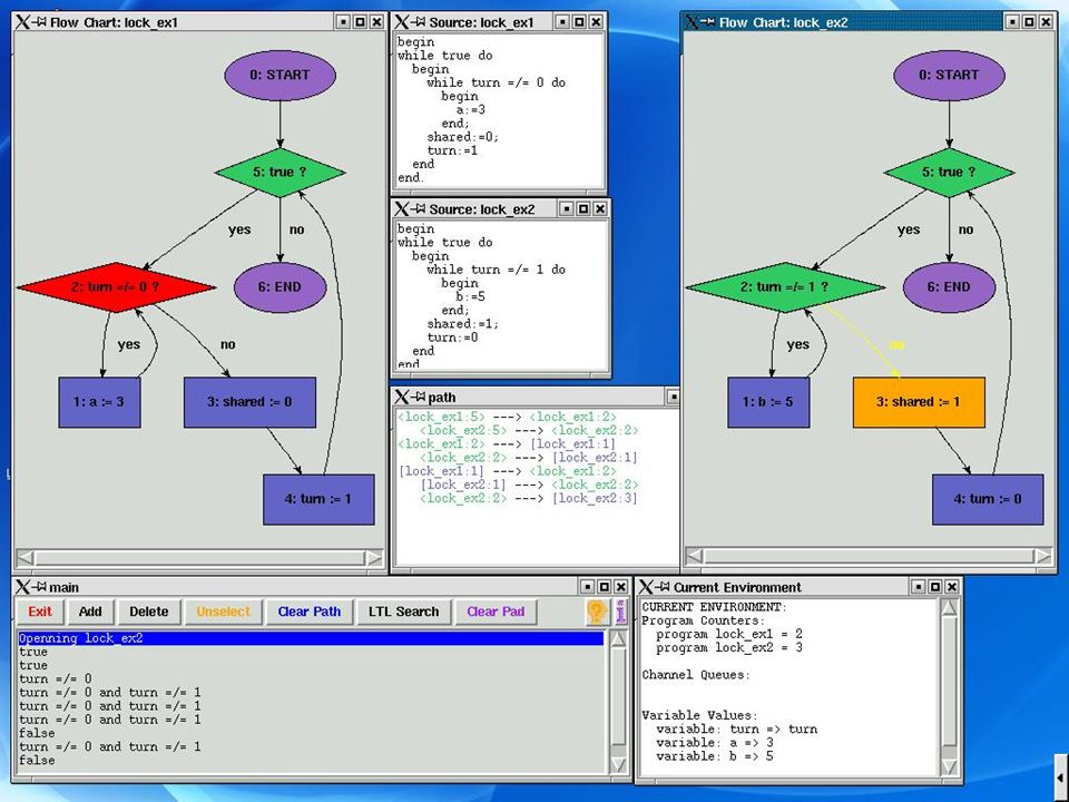


 for Microcontrollers>")


 Geometry (29%)>")


>")