1. MRes Course 2007-2008 THE ANALYSIS OF PSYCHOLOGICAL DATA

2. Personal details Colin Gray Room S16 (occasionally)
address:
Telephone: (27) 2233
Don’t hesitate to get in touch with me by if you have any queries or encounter any difficulties.

3. Four sessions
I shall be contributing 4 sessions to the MRes course: 2 in the first half-session, 2 in the second.
This week’s sessions amount to a selective REVISION and CONSOLIDATION of some elementary topics.
In March, I shall consider some more advanced methods.
There will be supporting PROJECTS.

4. SESSION 1 Basic statistics: some points and pitfalls

5. 1. GRAPHS

6. in Oxford Dictionary of Quotations, 1999.)
Proverb
‘One picture is worth
ten thousand words’
(Barnard, 1927, quoted
in Oxford Dictionary of Quotations, 1999.)

7. It’s not always true! Graphs can be difficult to understand.
They can also be highly misleading.

8. Keep your graphs simple!
A general principle:
Keep your graphs simple!

9. A research question
A drug is known to enhance the performance of tired people on a driving simulator.
It is suspected, however, that this drug may actually have a negative effect upon the performance of people who have had a good night’s rest.
We test this hypothesis with an experiment.

10. Factors
In the context of analysis of variance (ANOVA), a FACTOR is a set of related treatments, conditions or categories.
The ANOVA term ‘factor’ is a synonym for the term ‘independent variable’.

11. Experimental design

12. A two-factor between subjects factorial experiment
There are 2 treatment factors.
The presence of every combination of conditions ensures that the factors are independent or ORTHOGONAL: you can assess the effect of either independently of the other.
The hypothesis implies an INTERACTION between the two factors.

13. Results

14. Main effects and interactions

15. SPSS 15 SPSS frequently issues significant updates.
The University is now using SPSS 15.
The recommended textbook is based upon SPSS 15.

16. SPSS Data Editor In SPSS, there are two display modes:
1. Variable View. This contains information about the variables in your data set.
2. Data View. This contains your numerical data (referred to as ‘values’ by SPSS).
WORK IN VARIABLE VIEW FIRST, because that will make it much easier to enter your data in Data View.

17. Variable View

19. Data View

24. Levels of measurement
SPSS classifies data according to the LEVEL OF MEASUREMENT. There are 3 levels:
SCALE data, which are measures on an independent scale with units. Heights, weights, performance scores, counts and IQs are scale data. Each score has ‘stand-alone’ meaning.
ORDINAL data, which are ranks. A rank has meaning only in relation to the other individuals in the sample. It does not express the degree to which a property is possessed.
NOMINAL data, which are assignments to categories. (So-many males, so-many females.)

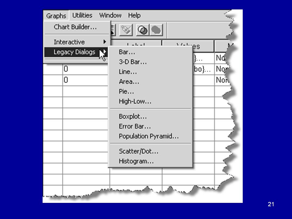
25. Graphics
The latest SPSS graphics require you to specify the level of measurement of the data on each variable.
The group code numbers are at the NOMINAL level of measurement, because they are merely CATEGORY LABELS.
Make the appropriate entry in the Measure column.

26. Specifying the level of measurement

28. BAR CHART

29. Questions What is a BAR CHART?
What is the difference between a bar chart and a HISTOGRAM?

30. A simple bar chart

32. Simple bar chart On the horizontal axis is the CATEGORY VARIABLE.
The ERROR BARS can represent multiples of either the standard deviation or the standard error.

33. A histogram

34. The difference
In the bar graph, the variable on the horizontal axis is QUALITATIVE or CATEGORICAL; in the histogram, the variable is CONTINUOUS.
In a histogram, the range is divided into arbitrary CLASS INTERVALS, upon which the bars rest.
This is why, in a histogram, there is no space between the bars – provided, of course, there are observations within adjacent class intervals.

35. Main effects
Returning to our experiment, the simple bar chart enables us to look at MARGINAL MEANS only, i.e., at MAIN EFFECTS.
We need a bar chart that pictures CELL MEANS so that we can examine the interaction.
A CLUSTERED bar chart enables us to depict an interaction.

36. A clustered bar chart

38. Clustered bar chart This is a CLUSTERED BAR CHART.
On the horizontal axis is the CATEGORY VARIABLE, Body State.
The CLUSTER VARIABLE is Drug.

39. Hypothesis confirmed
The chart shows clearly that the drug has indeed opposite effects upon fresh and tired drivers.
It improves the performance of TIRED drivers, but IMPEDES that of fresh drivers.

40. Error bars
The ERROR BARS assure us that the variance is reasonably homogeneous across groups.
Moreover, the differences among means are large compared with the standard errors.

41. Use simple graphics
Bar graphs can be over-embellished. The introduction of varying COLOURS AND TEXTURES and THREE-DIMENSIONAL EFFECTS can make it difficult to compare the heights of the bars.

42. Skyscrapers

44. An improvement? I find these SKYSCRAPERS distracting.
The artwork obscures the main point: the shaded bar is higher with the Tired group; the plain bar is higher with the fresh group.

45. Another experiment
An investigator runs an experiment in which the skilled performance of four groups of participants who have ingested four different supposedly performance-enhancing drugs is compared with that of a control or Placebo group.
When the data have been collected, the researcher enters them into SPSS and orders a one-way ANOVA.

46. Ordering a means plot

47. Output graph of the results

48. A false picture!
The table of means shows miniscule differences among the five group means.
The p-value of F is very high – unity to two places of decimals.
Nothing going on here!

49. A microscopic vertical scale
Only a microscopically small section of the scale is shown on the vertical axis: 10.9 to 11.4!
Even small differences among the group means look huge.

50. Putting things right
Double-click on the image to get into the Graph Editor.
Double-click on the vertical axis to access the scale specifications.

51. Putting things right …
Uncheck the minimum value box and enter zero as the desired minimum point.
Click Apply.

52. The true picture!

53. Look for the zero point The effect is dramatic.
The profile is now as flat as a pancake.
The graph now accurately depicts the results.
Always be suspicious of graphs that do not show the ZERO POINT on the VERTICAL SCALE.

54. 2. SMALL SAMPLES

55. Scarcity of data Sometimes our data are scarcer than we would wish.
This can create problems for the making of statistical tests such as the t-test, the chi-square test and the ANOVA.

56. Nominal data
A NOMINAL data set consists of records of membership of the categories making up QUALITATIVE VARIABLES, such as gender or blood group.
Nominal data must be distinguished from SCALAR, CONTINUOUS or INTERVAL data, which are measurements of QUANTITATIVE variables on an independent scale with units.
Nominal data sets merely carry potential information about the frequencies of observations in different categories.

57. A small set of nominal data
A medical researcher wishes to test the hypothesis that people with a certain type of body tissue (Critical) are more likely to show the presence of a potentially harmful antibody.
Data are obtained on 19 people, who are classified with respect to 2 attributes:
1. Tissue Type;
2. Whether the antibody is present or absent.

58. Contingency tables
When we wish to investigate whether an association exists between qualitative or categorical variables, the starting point is usually a display known as a CONTINGENCY TABLE, whose rows and columns represent the categories of the qualitative variables we are studying.

59. A contingency table
Is there an association between Tissue Type and Presence of the antibody?
The antibody is indeed more in evidence in the ‘Critical’ tissue group.

60. A disappointing result!
How disappointing! It looks as if we haven’t demonstrated a significant association.
Under the column headed ‘Asymp. Sig.’ is the p-value, which is given as

62. Significance level versus p-value
The significance (or alpha) level is a small, arbitrary probability (.05, .01) FIXED by convention.
The p-value (SPSS calls this ‘Sig.’) or SIGNIFICANCE PROBABILITY is calculated from the value of your test statistic.
It is the probability, under the null hypothesis, of obtaining a value at least as extreme as the one you have obtained.

63. The familiar chi-square formula

64. How it works
The formula works by comparing the OBSERVED frequencies (O) with the EXPECTED frequencies (E), which are calculated on the assumption that there is NO ASSOCIATION between Tissue Type and Presence of the antibody (the null hypothesis).

65. The true definition of chi-square
The familiar formula is NOT the DEFINING formula for chi-square.
Chi-square is NOT defined in the context of nominal data, but in terms of a normally distributed continous variable X thus…

66. True definition of chi-square
The true chi-square random variable on one degree of freedom is defined as the square of a standard normal variate Z.
Normally distributed variables are CONTINUOUS, that is, there are an infinite number of values between any two points on the scale.

67. An approximation
The familiar chi-square statistic is only APPROXIMATELY distributed as chi-square.
The approximation is good, provided that the expected frequencies E are ADEQUATELY LARGE.

68. The meaning of ‘Asymptotic’
The term ASYMPTOTIC denotes the LIMITING distribution of a statistic as the sample size approaches infinity.
The ‘asymptotic’ p-value of a statistic is its p-value under the ASSUMPTION that the statistic has the limiting distribution.
That assumption may be FALSE.

69. Goodness of the approximation…
In the SPSS output, the column headed ‘Asymp. Sig.’ contains a p-value calculated on the assumption that the approximate chi-square statistic behaves like the real chi-square statistic on the same degrees of freedom.
But underneath the table there is a warning about low frequencies, indicating that the ‘asymptotic’ p-value cannot be relied upon.

70. Exact tests
Fortunately, there are available EXACT TESTS, which do not use the approximate chi-square statistic.
There are the FISHER’S EXACT tests, designed by R. A. Fisher many years ago.
There are ‘brute force’ MONTE CARLO methods, which exploit the ability of modern computers to repeat, or ITERATE, massive computations again and again and thus ‘converge’ upon stable estimates.

71. A step ahead
In a real research situation, one line in an SPSS data set would contain data on only ONE person (‘case’).
We have taken a short-cut and started with a ready-made contingency table showing the counts of people in different categories. So one line in Data View refers to not one but several participants.
To process this data set, we need a special procedure.

72. In Variable View …
There are 3 elements in the contingency table: the two classifications; and the cell frequencies.
In SPSS, you will need to name 3 variables: 1. Tissue Type; 2. Presence/Absence of antibody; and 3. Count (frequency).
In Variable View, Name the three variables and assign labels (in the Values column) to the code numbers making up the various tissue groups.

73. Values In SPSS, a value is always A NUMBER.
With nominal variables, the Values column is used for attaching meaningful LABELS to arbitrary code numbers.
Arguably, the Values column in Variable View should be headed ‘Value Labels’.

75. Data View
The third variable, Count, contains the frequencies of occurrence and non-occurrence of the antibody in the different groups.
Thus in this artificial example, a single line in Dara View combines data from SEVERAL cases.
In this special situation, you must use the WEIGHT CASES procedure to warn SPSS; otherwise SPSS will assume that each line contains data from only one case.

76. Weighting the cases Select Weight Cases from the Data menu.
Complete the Weight Cases dialog by checking the Weight cases by button transferring Count to the Frequency Variable slot.
Click OK to weight the cases with their frequencies.

77. Selecting the chi-square test

78. Controlling the appearance of the output table
We want the 4 Tissue Types in the ROWS and Presence/Absence in the COLUMNS.
We can make that specification in the Crosstabs dialog.
We could have it the other way round: the ROWS could be Yes and No.

79. Controlling the tabulation

80. Ordering an exact test

82. Choosing extra statistics
We want the chi-square statistic and a measure of associative strength.
The chi-square statistic will not do as a measure of strength, because its value partially reflects the size of the data set.
Either the phi coefficient or Cramer’s V will do.
Back in the Crosstabs dialog, click Cells… and order percentages and expected frequencies.

84. A different result
The exact test has shown that we DO have evidence for an association between tissue type and incidence of the antibody.
The exact p-value is MARKEDLY LOWER than the aymptotic value.

85. Strength of the association
The chi-square statistic is unsuitable as a measure of the strength of an association, because it increases with the size of the data set.
Having asked for exact tests, we obtain exact p-values for phi and Cramer’s V.

86. 3. RELATED SAMPLES OF NOMINAL DATA

87. The scenario There is to be a debate on a contentious issue.
The debate is attended by 100 people. Each member of the audience is asked before and after the debate to write down whether they support the motion.

88. The researcher’s argument
The researcher argues that we are looking for an association between Response (Yes or No) and Time (Before, After).
There is an evident association: the proportion of Yes’s is markedly higher after the debate.
A chi-square test seems to confirm the association.

89. A misapplication of chi-square
The total frequency is 200, whereas there were only 100 participants.
A requirement for a chi-square test for an association is that each participant must contribute to the tally in only ONE cell of the contingency table.

90. Essential information
The researcher must keep track of each participant throughout the data-gathering exercise.
That permits the construction of the following table, which cannot be recovered from the previous table.
You cannot deduce the cell frequencies from the row and column marginal frequencies.

91. Another chi-square test??
We could run a chi-square test on this table, because each participant contributes to the tally in only one cell.
But if you were to do that, there would be nothing to report, because there is no evidence of an association.
Can we conclude that hearing the debate had no effect?

92. Wrong question!
We aren’t interested in whether there is an association between the way people vote before and after the debate.
We want to know whether hearing the debate has tended to CHANGE people’s views in one direction.

93. The McNemar test
The McNEMAR TEST only uses data on those participants who CHANGED THEIR VIEWS after hearing the debate.
The null hypothesis is that, in the population, as many people change positively as change negatively.
We note that while 13 people changed from Yes to No, 38 changed from No to Yes. That looks promising.

94. Association versus goodness-of fit
The tissue type example shows the use of the chi-square test to ascertain whether there is an ASSOCIATION between two variables.
Suppose we have nominal data on just ONE qualitative variable. For example, we learn that of 100 children, 60 prefer Toy A and 40 prefer Toy B.

95. Goodness-of-fit
The expected frequencies (E) show the null hypothesis, no-preference distribution.
The observed frequencies (O) show the observed distribution.
Does the expected distribution ‘fit’ the observed distribution?

96. Finding the McNemar test
The McNemar test is a test for goodness-of-fit, not a test for association.
It’s to be found in the Nonparametric Tests menu, under ‘2 Related Samples…’ .

97. Ordering a McNemar test
Transfer the two related variables (Before and After) to the right-hand panel.
Check the McNemar box.

98. The results
The McNemar test uses an approximate chi-square test of the null hypothesis that as many change from No to Yes as vice versa.
The null hypothesis is rejected. Now we have our evidence!
We write: χ2(1) = 11.29; p < .01 .
(Note: this chi-square statistic has one degree of freedom)

99. Correction for continuity
When there are only two groups (change to Yes, change to No), the chi-square statistic can only vary in jumps, rather than continuously.
The CORRECTION FOR CONTINUITY (Yates) attempts to improve the approximation to a real chi-square variable, which is continuous.
There has been much controversy about whether the correction for continuity is necessary.

100. Bernoulli trials
Is a coin ‘fair’: that is, in a long series of tosses, is the proportion of heads ½ ?
We toss the coin 100 times, obtaining 80 heads.
Arguably we have a set of 100 BERNOULLI TRIALS.
In a Bernoulli set, the outcomes of each trial can be divided into ‘success’ or ‘failure’, with probabilities p and 1 – p, respectively, which remain fixed over n independent trials.

101. Binomial probability model
Where you have Bernoulli trials, you can test the null hypothesis that the probability of a success is any specified proportion by applying the BINOMIAL PROBABILITY MODEL, which is the basis of the BINOMIAL TEST.
In our example, 51 people changed their vote and, of that number, 38 changed from No to Yes. Does that refute the null hypothesis that p = ½ ?

102. The binomial test There is no need to settle for an approximate test.
Set up your data like this.
Choose Data→Weight Cases and weight by Frequency.
Choose Analyze→Nonparametric Tests→Binomial and complete the dialog.

103. Completing the binomial dialog

104. The results The p-value is very small.
We have strong evidence that hearing the debate tended to change people’s views in the Yes direction more than in the No direction.

105. 4. T-TESTS AND SIGNIFICANCE TESTING

106. The caffeine experiment

107. Notational convention
We use Arabic letters to denote the statistics of the sample; we use Greek letters to denote PARAMETERS, that is, characteristics of the population.

108. The null hypothesis
The null hypothesis (H0) states that, in the population, the Caffeine and Placebo means have the same value.
H0: μ1 = μ2 15

109. The alternative hypothesis
The alternative hypothesis (H1) states that the Caffeine and Placebo means are not equal.

110. The test statistic
To test the null hypothesis, we shall need a TEST STATISTIC, in this case one which reflects the size of the difference between the sample means M1 and M2.
The t statistic fits the bill.

111. Independent samples
The Caffeine experiment yielded two sets of scores - one set from the Caffeine group, the other from the Placebo group.
There is NO BASIS FOR PAIRING THE SCORES.
We have INDEPENDENT SAMPLES.
We shall make an INDEPENDENT-SAMPLES t-test.

112. The t statistic
In the present example (where n1 = n2), the pooled estimate s2 of σ2 is simply the mean of the variance estimates from the two samples.

113. Denominator of t
The denominator of the t statistic is an estimate, from the data of the STANDARD ERROR OF THE DIFFERENCE BETWEEN MEANS.

114. Pooled variance estimate
The value of t
We do not know the supposedly constant population variance σ2.
Our estimate of σ2 is
Pooled variance estimate

115. Significance
Is the value 2.6 significant? Have we evidence against the null hypothesis?
To answer that question, we need to locate the obtained value of t in the appropriate SAMPLING DISTRIBUTION of t.
That distribution is identified by the value of the parameter known as the DEGREES OF FREEDOM.

116. Sampling distribution of t
There is a WHOLE FAMILY of t distributions.
To test H0, we must locate our value of t in the appropriate t distribution.
That distribution is specified by the DEGREES OF FREEDOM df, which is given by df = n1 +n2 – 2. In our example, df = – 2 = 38.

117. Degrees of freedom The df is the total number of scores minus two.
In our example, df = – 2 = 38.
WHETHER A GIVEN VALUE OF t IS SIGNIFICANT WILL DEPEND UPON THE VALUE OF THE DEGREES OF FREEDOM.

118. Appearance of a t distribution
A t distribution is very like the standard normal distribution.
The difference is that a t distribution has THICKER TAILS.
In other words, large values of t are more likely than large values of Z.
With large df, the two distributions are very similar.
Z~N(0, 1)
.95
.95
t(2)

119. Significance
To make a test of SIGNIFICANCE, we locate a CRITICAL region of values in the t distribution with 38 degrees of freedom.
A SIGNIFICANCE LEVEL or ALPHA-LEVEL is a small probability α, such as 0.05 and 0.01, fixed by convention. In psychology, the 0.05 level is generally accepted.
We locate the critical region in the tails of the t distribution, so that the probability of a value in EITHER one tail OR the other is α. In our case, α = The probability of a value in one PARTICULAR tail is α/2 =

120. The critical region
We shall reject the null hypothesis if the value of t falls within EITHER tail of the t distribution on 38 degrees of freedom.
To be significant beyond the .05 level, our value of t must be greater than OR less than –2.02.
(To be significant beyond the .01 level, our value of t must be greater than or less than –2.704.)

121. Pr of a value at least as small as yours
The p-value
The TOTAL blue area is the probability, under the null hypothesis, of getting a value of t at least as extreme as your value.
If the p-value is less than .05, you are in the critical region, and your value of t is significant beyond the .05 level.
Pr of a value at least as small as yours

122. The sign of t The sign of t is IRRELEVANT.
If t is negative, it’s in the lower tail: if it’s positive, it’s in the upper tail.
In either case, the p-value is the TOTAL blue area, because an extreme value in EITHER direction is evidence against the null hypothesis.

123. Direction of subtraction in the t test
The value of t is based upon the difference between means M1 – M2.
If the first mean is larger than the second, the difference (and t) will be positive.
When in the t-test procedure, you complete the Define Groups dialog, the mean for the group entered second will be subtracted from the mean for the group entered first.
We entered the values in the order: 1, 0, ensuring that the Placebo mean would be subtracted from the Caffeine mean.

124. Avoiding the negative sign
By entering the Caffeine mean first, we ensure that the sign of t is positive.
Had the Placebo mean had been larger, the sign of t could still have been kept positive by entering that mean first when defining the groups in the t-test dialog.
That’s fine – a difference in EITHER direction can lead to rejection of the null hypothesis.

125. Result of the t test
The p-value of 2.6 is .01 (to 2 places of decimals).
Our t test has shown significance beyond the .05 level.
But the p-value is greater than .01, so the result, although significant beyond the .05 level, is not significant beyond the .01 level.

126. The p-value is expressed to two places of decimals
Your report
“The scores of the Caffeine group (M = 11.90; SD = 3.28) were higher than those of the Placebo group (M = 9.25; 3.16). With an alpha-level of 0.05, the difference is significant: t(38) = 2.60; p = ”
The p-value is expressed to two places of decimals
degrees of freedom
value of t

127. Representing very small p-values
Suppose, in the caffeine experiment, that the p-value had been very small indeed. (Suppose t = 6.0). The computer would have given your p-value as ‘.000’. NEVER WRITE, ‘p = .000’. This is unacceptable in a scientific article.
Write, ‘p < .01’.
You would have written the result of the test as
‘ t(38) = 6.0; p < .01’ .

128. Directional hypotheses
The null hypothesis states simply that, in the population, the Caffeine and Placebo means are equal.
H0 is refuted by a sufficiently large difference between the means in EITHER direction.
But some argue that if our scientific hypothesis is that Caffeine improves performance, we should be looking at differences in only ONE direction.

129. One-tail tests
Suppose are only interested in the possibility of a difference in ONE DIRECTION.
You would locate the CRITICAL REGION for your test in ONE tail of the distribution.
0.025
(2.5%)
0.025
(2.5%)
0.05
(5%)

130. A strong case for a one-tailed test
Neurospsychologists often want to know whether a score is so far below the norm that there is evidence for brain damage.
Arguably, in this case, a one-tailed test is justified because it seems unlikely that brain damage could actually IMPROVE performance.
But note that, on a one-tail test, you only need a t-value of about 1.7 for significance, rather than a value of around 2.0 for a two-tail test. (The exact values depend upon the value of the df.
So, on a one-tail test, it’s easier to get significance IN THE DIRECTION YOU EXPECT.
For this reason, many researchers (and journal editors) are suspicious of one-tail tests.

131. 5. TYPE I AND TYPE II ERRORS

132. Type I error Suppose the null hypothesis is true.
If you keep sampling a large number of times, every now and again (in 5% of samples), you will get a value of t in one of the tail areas (the critical region) and reject the null hypothesis.
You will have made a TYPE I ERROR.
The probability of a Type I error is the significance level, which is also termed the ALPHA-LEVEL, because it is also the probability of a Type I error.

133. Type II error
A Type II error is said to occur when a test fails to show significance when the null hypothesis is FALSE.
The probability of a Type II error is symbolised as β, and is also known as the TYPE II ERROR RATE or BETA RATE.

134. The beta rate The light-grey area is part of the critical region.
Any value of t outside the tail of the H0 distribution is insignificant.
The dark area is the probability that the null hypothesis will be accepted, even though it is false.
This is the BETA RATE.
α/2
Real difference

135. 6. POWER

136. Power
The POWER of a statistical test is the probability that the null hypothesis will be refected, given that it is FALSE.

137. Power
The power of the statistical test is the area under the H1 distribution to the right of the dark-grey area.
This is the POWER of the test.
α/2
Real difference

138. Power and the beta rate
Since the entire area under either curve is 1, the area in the H1 distribution to the right of the dark area (the power) is 1 – β.
α/2
Real difference

139. Increasing the power
By REDUCING the beta-rate, you INCREASE the power of the test, because beta-rate + power = 1.

140. Type 1 and type 2 errors: power
Type I error
Pr = α
Type II error
Pr = β

141. A change in emphasis
Traditionally, the emphasis had been on controlling Type I errors.
This is achieved by insisting upon statistical significance.
Even more control would be achieved by adopting the 0.01 significance level, rather than the 0.05 level.
So why not fix alpha at 0.01, rather than 0.05?

142. Significance level and the beta-rate
Suppose you decide upon a smaller significance level (lower figure).
The probability of a type II error (green) increases.
The power (P) decreases. P β β P

143. The need to strike a balance
Adopting the 0.01 level reduces the Type I error rate.
But that INCREASES the Type II error rate and REDUCES the power of the test.
It is now considered that, in the past, there was insufficient concern with high beta-rates and low power.
The 0.05 level is thought to achieve the right BALANCE between Type I and Type II errors.

144. Power and sample size
Increasing the sample size reduces the overlap of the sampling distributions under H0 and H1.
The beta-rate is reduced and so the power increases.
Small samples
Large samples
Real difference

145. Small samples
Small samples bring the distributions together, increase the size of the dark-grey area and reduce the power of the test.
Large samples separate the distributions, reduce the dark-grey area and increase the power of the test.
α/2
Real difference

146. Factors affecting the Type II error rate
An insufficiency of data (too few participants) means that the sampling distributions under H0 and under H1 overlap too much and most of the H1 distribution lies below the critical value for rejection of H0.
A similar effect arises from unreliable data, which inflate random variation and increase the overlap.
Finally, as we have seen, fixing a lower significance level (0.01 rather than 0.05) also increases the beta-rate.

147. How much power do we need?
Cohen (1988) observed a general tendency for psychologists to be preoccupied with avoiding Type I errors and insufficiently concerned with the possibility of Type II errors.
Most tests had insufficient power. Power levels as low as 0.05 were not uncommon.
A MINIMUM POWER OF 0.75 IS RECOMMENDED.

148. 7. EFFECT SIZE

149. A ‘substantial’ difference?
We obtained a difference between the Caffeine and Placebo means of (11.90 – 9.25) = 2.75 score points.
If we take the spread of the scores to be the average of the Caffeine and Placebo SDs, we have an average SD of about 3.25 score points.
So the means of the Caffeine and Placebo groups differ by about .8 SD.

150. Measuring effect size: Cohen’s d statistic
In our example, the value of Cohen’s d is 2.75/3.25 = .8 .
Is this a ‘large’ difference?

151. Levels of effect size
On the basis of scrutiny of a large number of studies, Jacob Cohen proposed that we regard a d of .2 as a SMALL effect size, a d of .5 as a MEDIUM effect size and a d of .8 as a LARGE effect size.
So our experimental result is a ‘large’ effect.
When you report the results of a statistical test, you are now expected to provide a measure of the size of the effect you are reporting.

152. 8. SHOULD WE MAKE ONE-TAILED TESTS?

153. One-tail tests
Suppose we are only interested in the possibility of a difference in ONE DIRECTION.
Some argue that we should locate the critical region for our test in one tail only of the t distribution.
The critical value of t is now lower.
0.025
(2.5%)
0.025
(2.5%)
0.05
(5%)

154. Another result
Suppose that the mean score of the Caffeine group had been, not 11.90, but
In other words, the Caffeine and Placebo means differ by only 1.72 points, rather than 2.65 points, as in the original example.
The value of t is now 1.69, which is the critical value on a one-tail test.

155. Report of the one-tailed test
“The scores of the Caffeine group (M = 10.97; SD = 3.28) were significantly higher than those of the Placebo group (M = 9.25; 3.16): t(38) = 1.69; p = .05 (one-tailed) .”
The p-value is expressed to two places of decimals
degrees of freedom
value of t

156. Advantage of the one-tailed test
Our t value of 1.69 would have failed to achieve significance on the two-tailed test, since the critical value was
On the one-tailed test, however, t is in the critical region and the null hypothesis is rejected.

157. More power
In locating the entire critical region in the upper tail of the H0 distribution, we increase the light-grey area and reduce the dark-grey area.
In order words, we increase the POWER of the test to reject H0.
Real difference

158. An unexpected result
Now suppose that, against expectation, the Placebo group had outperformed the Caffeine group.
The mean for the Caffeine group is 9.25 and that for the Placebo group is
Were we to subtract the smaller mean from the larger (as in the traditional approach), we should obtain t =
On a two-tailed test, this is in the critical region (p <.05) and we should reject the null hypothesis.

159. The null hypothesis

160. Direction of subtraction
The direction of subtraction is now crucial.
You MUST subtract the Placebo mean from the Caffeine mean.
Only a POSITIVE value of t can falsify the directional null hypothesis.

161. One-sided p-value
In the one-tailed test, the p-value is ONE-SIDED, that is, it is the probability, under the one-sided null hypothesis, that the Caffeine mean would have been at least as LARGE as the one we obtained.

162. The one-sided p-value
The one-sided p-value is the entire area under the curve to the right of your value of t. This includes the black area.
That area is
-2.02
Your value of t.

163. Report of the one-tail test
“The scores of the Caffeine group (M = 9.25; SD = 3.16) were not significantly higher than those of the Placebo group (M = 10.20; SD = 3.28): t(38) = ; p = (one-tailed) .”

164. Changing horses
Oh dear! I have made a two-tailed tests and I haven’t got significance! The RAE is fast approaching and I won’t get my paper published!
I know: I’ll make a one-tail test instead.
There we are, the result is significant!
Problem solved!

165. The true Type I error rate.
If you follow that practice, your true Type I error rate is now the black area (0.05) PLUS the area in the lower tail (0.025). This is = 0.075, a level many feel is too high.
0.025

166. One-tailed tests?
I have concerns about the making of one-tailed tests.
There are two reasons for this.
You could find yourself unable to report a surprising result.
Many journal editors are suspicious of one-tail tests – and with good reason.

167. A special situation
Neurospsychologists often want to know whether a score is so far BELOW the norm that there is evidence for brain damage.
They want to establish a cut-off point below which a score is deemed to be indicative of impairment.
A one-tail test is appropriate there.
My OWN VIEW is that one-tail tests are seldom justified in RESEARCH, as opposed to clinical practice.

168. 9. HOW MANY PARTICIPANTS SHALL I NEED?

169. How many participants?
That depends upon the minimum effect size that you want to pick up with your significance tests.
You also want to make sure your power is at least at the 0.75 level.
You can obtain the number of participants necessary by looking up tables (Cohen 1988; Clark-Carter, 2004).

170. Books with power tables
Clark-Carter, D. (2004). Quantitative psychological research: a student’s handbook (2nd ed.). Hove: Psychology Press.
Cohen, J. (1988). Statistical power analysis for the behavioral sciences (2nd ed.). Hillsdale, NJ: Lawrence Erlbaum.

171. Using the Web
The Web is a very useful source of up-to-date information on all statistical topics, including power and effect size.
Use the Google search engine.
Their address is
Use the phrases ‘statistical power’ and ‘effect size’.

172. Software
Software is available for finding the numbers of participants you will need to make a test at a specified level of power.
An example is G*Power (Erdfelder et al., 1996).
G*Power is available on the Web.

173. The Google window

174. Useful information on the Web

175. The G-power opening window

176. Using G-Power
You can choose the ‘a priori’ option to find out how many participants you need to achieve a power of .95 of rejecting the null hypothesis for a medium effect on a one-tail test.
You need 176 participants!
That’s why we usually settle for a power level of 0.75!
You fill in these values
The answers

177. 10. ANOVA

178. A one-factor, between subjects experiment

179. Results of a one-factor, between subjects experiment
raw scores
grand mean

180. Statistics of the results
group (cell) means
Group (cell) variances
group (cell) standard deviations

181. The null hypothesis
The null hypothesis states that, in the population, all the means have the same value.
In words, the null hypothesis states that none of the drugs has any effect.

182. The alternative hypothesis
The alternative hypothesis is that, in the population, the means do NOT all have the same value.
There are MANY POSSIBILITIES for H1.
The rejection of H0 does not imply that any one of these possibilities is true.

183. The one-way ANOVA
The ANOVA of a one-factor BETWEEN SUBJECTS experiment is also known as the ONE-WAY ANOVA.
The one-way ANOVA must be sharply distinguished from the one-factor WITHIN SUBJECTS (or REPEATED MEASURES) ANOVA, which is appropriate when each participant is tested under every condition.
The between subjects and within subjects ANOVAs are predicated upon different statistical MODELS.

184. There are some large differences among the five treatment means, suggesting that the null hypothesis is false.

185. Variance or Mean Square (MS)
In ANOVA, the numerator of a variance estimate is known as a SUM OF SQUARES (SS). The denominator is known as the DEGREES OF FREEDOM (df). The variance estimate itself is known as a MEAN SQUARE (MS), so that MS = SS/df .

186. Accounting for variability
grand mean
Accounting for variability
total deviation
between groups deviation
within groups deviation
The building block for any variance estimate is a DEVIATION of some sort.
The TOTAL DEVIATION of any score from the grand mean (GM) can be divided into 2 components: 1. a BETWEEN GROUPS component; 2. a WITHIN GROUPS component.

187. Example of the breakdown
The score, the group mean and the grand mean have been ringed in the table.
This breakdown holds for each of the fifty scores in the data set.
score
grand mean
group mean

188. Breakdown (partition) of the total sum of squares
If you sum the squares of the deviations over all 50 scores, you obtain an expression which breaks down the total variability in the scores into BETWEEN GROUPS and WITHIN GROUPS components.

189. How ANOVA works
The variability BETWEEN the treatment means is compared with the average spread of scores around their means WITHIN the treatment groups.
The comparison is made with a statistic called the F-RATIO.

190. The F ratio

191. What F is measuring
If there are differences among the population means, the numerator will be inflated and F will increase.
If there are no differences, the two MS’s will have similar values and F will be close to 1.
error + real differences
error only

192. What F is measuring
If the null hypothesis is true, the values of MSbetween and MSwithin will be similar, because both variance estimates merely reflect individual differences and random variation or ERROR.
If so, the value of F will be around 1.
If the null hypothesis is false, real differences among the population means will inflate the value of MSbetween but the value of MSwithin will be unaffected.
The result will be a LARGE value of F.

193. Range of variation of F
The F statistic is the ratio of two sample variances.
A variance can take only non-negative values.
So the lower limit for F is zero.
There is no upper limit for F.

194. Repeated sampling Suppose the null hypothesis is true.
Imagine the experiment were to be repeated thousands and thousands of times, with fresh samples of participants each time.
There would be thousands and thousands of data sets, from each of which a value of F could be calculated.

195. Sampling distribution
To test the null hypothesis, you must be able to locate YOUR value of F in the population or DISTRIBUTION of such values.
The distribution of a statistic is known as its SAMPLING DISTRIBUTION.
To specify the correct distribution of F (or any other test statistic), you must assign values to properties known as PARAMETERS.

196. Parameters of F
Recall that the t distribution has ONE parameter: the DEGREES OF FREEDOM (df ).
The F distribution has TWO parameters: the degrees of freedom of the between groups and within groups mean squares, which we shall denote by dfbetween and dfwithin, respectively.

197. Rule for finding the degrees of freedom
There’s a useful rule for finding the degrees of freedom of a statistic.
Take the number of independent observations and subtract the number of parameters estimated.
The sample variance of n scores is based upon n independent observations. But to obtain the deviations, we need an estimate of ONE parameter, namely, the mean.
So the degrees of freedom of the sample variance is n – 1, not n.

198. Rule for obtaining the df

199. Degrees of freedom for the one-way ANOVA mean squares
The degrees of freedom df of a sum of squares is the number of independent values (scores, means) minus the number of parameters estimated.
The SSbetween is calculated from 5 group means, but ONE parameter (the grand mean) has been estimated.
Therefore dfbetween = 5 – 1 = 4.

200. Degrees of freedom …
The SSwithin is calculated from the scores of the 50 participants in the experiment; but the group mean is subtracted from each score to produce a deviation score.
There are 5 group means.
The dfwithin = 50 – 5 = 45.

201. Calculating MSwithin
In the equal-n case, we can simply take the mean of the cell variance estimates.
MSwithin = ( )/5 =48.36/5 = 9.67

202. Finding MSbetween

203. The value of MSwithin , since it is calculated only from the variances of the scores within groups and ignores the values of the group means. It reflects only RANDOM ERROR.

204. The value of the MSbetween , since it is calculated only from the MEANS, reflects random error, PLUS any real DIFFERENCES among the population means that there may be.

205. Degrees of freedom of the two mean squares
The degrees of freedom of MSbetween is the number of treatment groups minus 1. (One parameter estimated: the grand mean.)
The degrees of freedom of MSwithin is the total number of scores minus the number of treatment groups. (Five parameters are estimated: the five group means.)

206. The correct F distribution
We shall specify an F distribution with the notation F(dfbetween, dfwithin).
We have seen that in our example, dfbetween = 4 and dfwithin = 45.
The correct F distribution for our test of the null hypothesis is therefore F(4, 45).

207. The distribution of F(1, 45)
F distributions are POSITIVELY SKEWED, i.e., they have a long tail to the right.
However, the shape of F varies quite markedly with the values of the df.

208. The distribution of F(4, 45)

209. Percentiles
A PERCENTILE is the VALUE or SCORE below which a specified percentage or proportion of the distribution lies.
The 30th percentile is the value below which 30% of the distribution lies.
The 70th percentile is the value below which 70% of scores lie.

210. The 30th and 70th percentiles
(0.70)
0.30
30th percentile
0.70
(0.30)
70th percentile

211. The median is the 50th percentile
0.50
0.50
50th percentile
(median)

212. The critical region
The critical region lies in the UPPER TAIL of this F distribution.
If we set the significance level at .05, the value of F must be at least 2.58.
The value 2.58 is the 95th Percentile of the distribution F(4, 45).

213. The F distribution
F(dfbetween, dfwithin) = F(4, 45)
.05
.95 F
95th percentile = 2.58
An F distribution is asymmetric, with an infinitely long tail to the right.
The critical region lies above the 95th percentile which, in this F distribution, is 2.58.

214. The ANOVA summary table
F large, nine times larger than unity, the expected value from the null hypothesis and well over the critical value 2.58.
The p-value (Sig.) <.01. So F is significant beyond the .01 level.
Do not write the p-value as ‘.000’.
Write this result as follows: ‘with an alpha-level of .05, F is significant: F(4, 45) = 9.09; p <.01’.
Notice that SStotal= SSbetween groups + SSwithin groups
The same breakdown applies to the degrees of freedom also.

215. The two-group experiment

216. ANOVA or t-test?
We can compare the two means by using an independent-samples t-test.
But what would happen if, instead of making a t test, we were to run an ANOVA to test the null hypothesis of equality of the means?

217. The two-group case: comparison of ANOVA with the t-test
Observe that F = t2 .
Observe also that the p-value is the same for both tests.
The ANOVA and the independent-samples t test are EXACTLY EQUIVALENT and result in the same decision about the null hypothesis.

219. Equivalence of F and t in the two-group case
When there are only two groups, the value of F is the square of the value of t.
So if t is significant, then so is F and vice versa.

220. Explanation

221. Effect size in ANOVA
The greater the differences among the means, the greater will be the proportion of the total variability that is ‘explained’ or accounted for by SSbetween.
This is the basis of the oldest measure of effect size in ANOVA, which is known as ETA SQUARED (η2).

222. Eta squared
Eta squared (also known as the CORRELATION RATIO) is defined as the ratio of the between groups and within groups mean squares.
It’s theoretical range of variation is from zero (no differences among the means) to unity (no variance in the scores of any group, but different values in different groups).
In our example, η2 = .447

223. Comparison of eta squared with Cohen’s d

225. Positive bias of eta squared
The correlation ratio (eta squared) is positively biased as an estimator.
Imagine you were to have huge numbers of participants in all the groups and calculate eta squared. This is the population value, which we shall term ρ2 (rho squared).
Imagine your own experiment (with the same numbers of participants) were to be repeated many times and you were to calculate all the values of eta squared.
The mean value of eta squared would be higher than that of rho squared.

226. Removing the bias: omega squared
The measure known as OMEGA SQUARED corrects the bias in eta squared.
Omega squared achieves this by incorporating degrees of freedom terms.

227. Adjusted R2 SPSS does not offer omega squared in its output.
SPSS calculates another measure of effect size that corrects the positive bias in eta squared.
The measure is termed ADJUSTED R2.
I shall give a fuller explanation of that statistic in my second session, on Wednesday.

228. Recommended reading
For a thorough and readable coverage of elementary (and not so elementary) statistics, I recommend …
Howell, D. C. (2007). Statistical methods for psychology (6th ed.). Belmont, CA: Thomson/Wadsworth.

229. For SPSS
Kinnear, P. R., & Gray, C. D. (2007). SPSS 15 for windows made simple. Hove and New York: Psychology Press.
In addition to being a practical guide to the use of SPSS, this book also offers informal explanations of many of the techniques.

230. For these sessions …
I suggest you might read Kinnear & Gray, Chapter 7 (for Monday’s session) and Chapter 12 (for Wednesday).