1. SESSION 2 ANOVA and regression

2. Only the starting point
In ANOVA, the rejection of the null hypothesis leaves many questions unanswered.
Further analysis is needed to pinpoint the crucial patterns in the data.
So, unlike the t test, the ANOVA is often just the first step in what may be quite an extensive statistical analysis.

3. Comparisons among the five treatment means

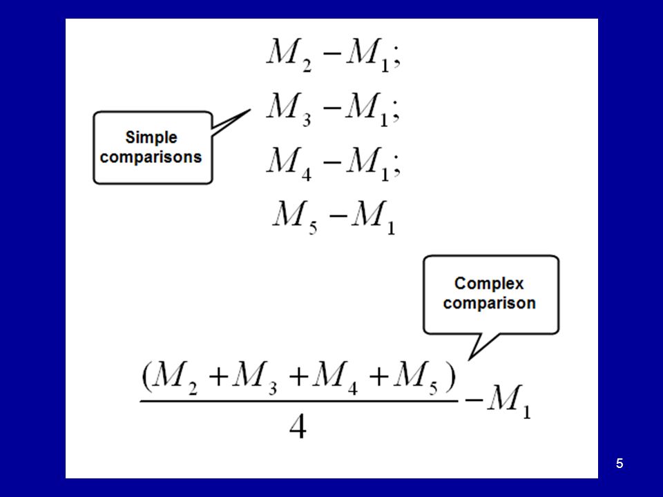
4. Simple and complex comparisons
You might want to make SIMPLE COMPARISONS between the mean for each of the four drug conditions and the Placebo mean.
Or you might want to compare the Placebo mean with the mean of the four drug means. This is a COMPLEX COMPARISON.

6. Non-independence of comparisons
The simple comparison of M5 with M1 and the complex comparison are not independent.
The value of M5 feeds into the value of the average of the means for the drug groups.

7. Systems of comparisons
With a complex experiment, interest centres on SYSTEMS of comparisons.
Which comparisons are independent or ORTHOGONAL?
What is the probability, under the null hypothesis, that at least one comparison will show significance?
How much variance can we attribute to different comparisons?

8. The crumpled paper fallacy
We owe this to Thouless.
Uncrumple a piece of paper.
The wrinkles are unique.
Therefore, they are statistically significant.
Data sets from complex experiments may, ex post facto, show all manner of interesting patterns.
Inferences from such patterns are dangerous.

9. Over-analysis?
You have run a complex experiment and submitted a paper to a journal.
Your reviewers will need to be convinced that what you are reporting isn’t just a chance pattern thrown up by sampling error.
You may well be asked to specify orthogonal comparisons and test them for significance.

10. Linear functions
Y is a linear function of X if the graph of Y upon X is a straight line.
For example, temperature in degrees Fahrenheit is a linear function of temperature in degrees Celsius.

11. F is a linear function of C
Degrees Fahrenheit P Q
Intercept → 32
(0, 0)
Degrees Celsius

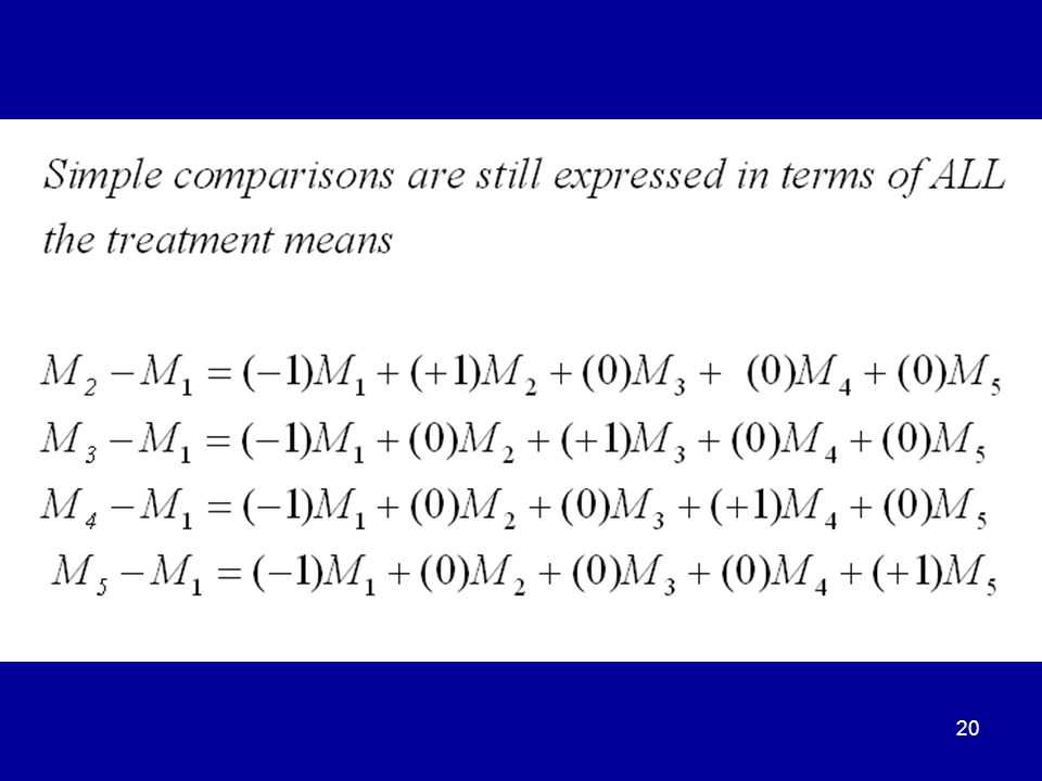
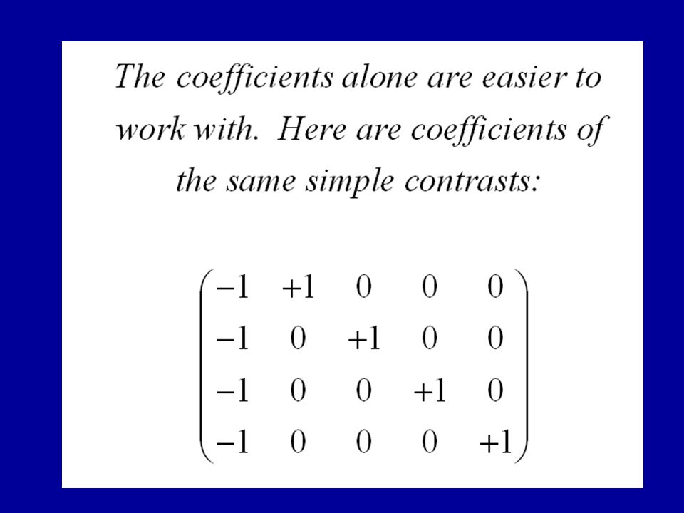
14. Linear contrasts
Any comparison can be expressed as a sum of terms, each of which is a product of a treatment mean and a coefficient such that the coefficients sum to zero.
When so expressed, the comparison is a LINEAR CONTRAST, because it has the form of a linear function.
It looks artificial at first, but this notation enables us to study the properties of systems of comparisons among the treatment means.

17. More compactly, if there are k treatment groups, we can write

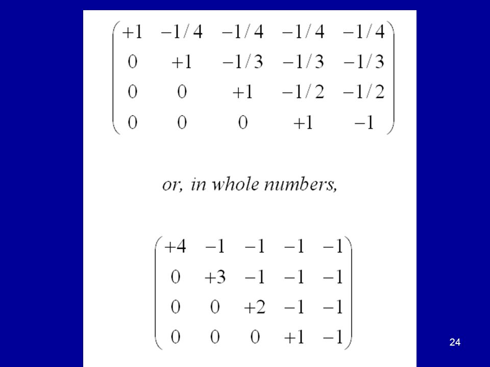
22. Helmert contrasts
Compare the first mean with the mean of the other means.
Drop the first mean and compare the second mean with the mean of the remaining means. Drop the second mean.
Continue until you arrive at a comparison between the last two means.

23. Helmert contrasts… Our first contrast is 1, -¼, -¼, -¼, -¼
Our second contrast is
0, 1, -⅓ , -⅓, -⅓
Our third contrast is
0, 0, 1, -½, -½
Our fourth is
0, 0, 0, 1, -1

25. Orthogonal contrasts
The first contrast in no way constrains the value of the second, because the first mean has been dropped.
The first two contrasts do not affect the third, because the first two means have been dropped.
This is a set of four independent or ORTHOGONAL contrasts.

26. The orthogonal property
The sum of the products of corresponding coefficients in any pair of rows is zero.
This means that we have an ORTHOGONAL contrast set.

27. Size of an orthogonal set
In our example, with five treatment means, there are four orthogonal contrasts.
In general, for an array of k means, you can construct a set of, at most, k-1 orthogonal contrasts.
In the present ANOVA example, k = 5, so the rule tells us that there can be no more than 4 orthogonal contrasts in the set.
Several different orthogonal sets, however, can often be constructed for the same set of means.

28. Accounting for variability
grand mean
Accounting for variability
total deviation
between groups deviation
within groups deviation
The building block for any variance estimate is a DEVIATION of some sort.
The TOTAL DEVIATION of any score from the grand mean (GM) can be divided into 2 components: 1. a BETWEEN GROUPS component; 2. a WITHIN GROUPS component.

29. Breakdown (partition) of the total sum of squares
If you sum the squares of the deviations over all 50 scores, you obtain an expression which breaks down the total variability in the scores into BETWEEN GROUPS and WITHIN GROUPS components.

30. Contrast sums of squares
We have seen that in the one-way ANOVA, the value of SSbetween reflects the sizes of the differences among the treatment means.
In the same way, it is possible to measure the importance of a contrast by calculating a sum of squares which reflects the variation attributable to that contrast alone
We can use an F statistic to test each contrast for significance.

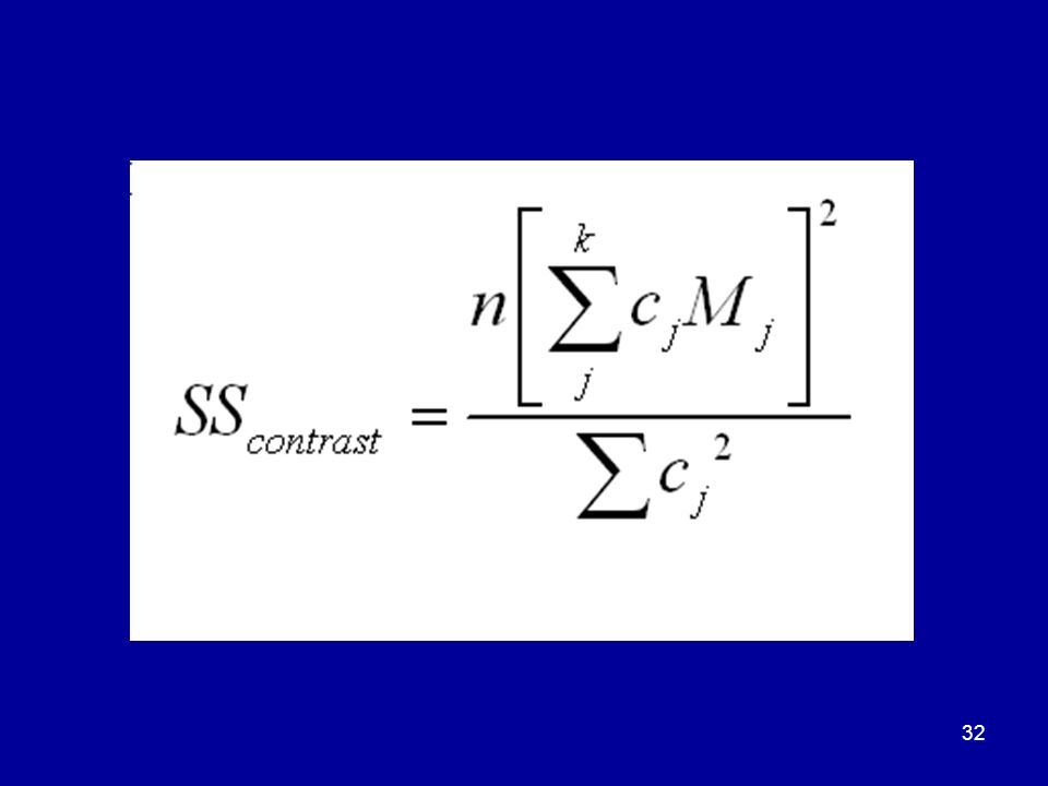
31. Formula for a contrast sum of squares

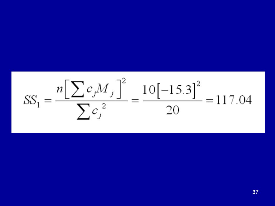
33. Here, once again, is our set of Helmert contrasts, to which I have added the values of the five treatment means

40. Testing a contrast sum of squares for significance

41. Two approaches A contrast is a comparison between two means.
You can therefore run a one-way, 2-group ANOVA.
Or you can use a t-test.
The tests are equivalent.

42. Degrees of freedom of a contrast sum of squares
A contrast sum of squares compares two means.
A contrast sum of squares, therefore, has ONE degree of freedom, because the two deviations from the grand mean sum to zero.

48. Contrasts with SPSS Two approaches:
The simpler is through the One-Way option in the Compare Means menu.
The General Linear Model, however, provides many more useful statistics.
I suggest you begin by exploring contrasts with the One-Way procedure first, then move on to the General Linear Model menu.

51. Contrasts with SPSS
The coefficients must be integers

53. Our Helmert contrasts Each ringed item is a MEAN.
In the top row, the Placebo mean is compared with the mean of the drug means.
In the third row, the mean for Drug B is compared with the mean of the means for Drug C and Drug D.

54. Summary A contrast is a comparison between two means.
The contrasts can therefore be tested with either F or t. (F = t2.)
The contrast sums of squares sum to the value of SSbetween.

56. Heterogeneity of variance
The lower part of the table shows the results of tests of the same contrasts when homogeneity of variance is not assumed.
Notice that the degrees of freedom have lower values.

57. Non-orthogonal contrasts
Contrasts don’t have to be independent.
For example, you might wish to compare each of the four drug groups with the Placebo group.
What you want are SIMPLE CONTRASTS.

58. Simple contrasts These are linear contrasts – each row sums to zero.
But they are not orthogonal – with some pairings, the sum of products of corresponding coefficients is not zero.

59. Simple contrasts with SPSS
Here are the entries for the first contrast, which is between the Placebo and Drug A groups.
Below that are the entries for the final contrast between the Placebo and Drug D groups.

60. The results
In the column headed ‘Value of Contrast’, are the differences between pairs of treatment means.
For example, Drug A mean minus Placebo mean = = Drug D – Placebo = – 8.00 = 5.00.

61. Trend analysis
Sometimes the factor (independent variable) may be quantitative and continuous.
The theory of contrasts can be extended to study trends in the relationship between the factor and the dependent variable.
The following slides outline the procedure.

62. Polynomials
A POLYNOMIAL is a sum of terms, each of which is a product of a constant and a power of the same variable.
The highest power n is the DEGREE of the polynomial.

63. Graphs of some polynomials
QUADRATIC
LINEAR
CUBIC
QUARTIC

64. Fitting points with polynomials
A first-order polynomial (line) does not change direction at all. But you can adjust the constants to fit any TWO points.
A second-order polynomial (parabola) changes direction ONCE and can be fitted to any THREE points.
A third-order polynomial changes direction TWICE and can be fitted to any FOUR points.

65. Fitting points with polynomials…
In general, any k points can be fitted perfectly by a polynomial of order k – 1.

66. LINEAR
QUADRATIC
CUBIC

67. Another drug experiment
In the drug experiment, the independent variable (or factor) comprised a set of five qualitatively different conditions.
There was no intrinsic ordering of the categories. The order in which the variables appeared in Data View was entirely arbitrary.
Now suppose that the five groups vary in the extent to which the same drug was present.
The Placebo, A, B, C and D groups have dosages of 0, 10, 20, 30 and 40 units of the drug, respectively.
The five groups are now ordered with respect to a CONTINUOUS INDEPENDENT VARIABLE.

68. A linear trend There is evidence of a linear TREND in these data.
The pattern, however, is imperfect – other trends (e.g. quadratic) may be present as well. On the other hand, the irregularity may reflect random error.

69. Capturing the linear trend
Consider the linear contrast
If we plot these values against X (the concentration of the drug), we shall have the graph of a straight line.
LINEAR

70. Polynomial coefficients
The coefficients in this contrast are actually values of the polynomial
y = x – 3
The sum of squares of this contrast captures or reflects the linear trend in the data.

71. Orthogonal polynomial contrasts
Here is a set of orthogonal contrasts.
The values in each row are values of one polynomial for various values of X, the continuous independent variable.
The top row is a first degree (linear) polynomial, the next row is a second degree (quadratic) polynomial and so on.

72. Trend analysis
Although the entries in a row are values of the same polynomial (whether linear or not), they are still the coefficients of a linear contrast: they sum to zero; moreover, the products of the corresponding coefficients also sum to zero. We have an ORTHOGONAL SET of contrasts.
Associated with each contrast is a sum of squares which captures that particular trend in the data.
The contrasts are tested in the usual way.

73. Ordering a linear polynomial contrast
Specify a linear (1st degree) polynomial
You must check the Polynomial box and specify the order of the polynomial.
Orthogonal polynomial sets are obtainable from tables in statistics books, such as Howell (2007), which provide orthogonal sets for sets of means of various sizes.
You must check the Polynomial box

74. Ordering a quadratic polynomial contrast
Specify a 2nd degree (quadratic) polynomial
You must now specify a Quadratic (2nd degree) polynomial.
The coefficients are entered in the usual way.

75. A trend analysis The relevant results are ringed.
You can see that only the linear trend is significant.
This formal analysis confirms the appearance of the profile plot.

76. Partition of the between groups sum of squares
Since we have an orthogonal set of contrasts, their sums of squares sum to the ANOVA between groups sum of squares.

77. Deviations in the ANOVA table
The DEVIATION sum of squares is what remains of SSbetween when the last contrast sum of squares has been subtracted.
Each deviation has one degree of freedom fewer than the previous deviation (if there is one).

78. The deviations
The first deviation SS (with df = 3) is obtained by subtracting the linear SS from SSbetween
The second deviation has df = 2. Both the linear and the quadratic trends have now been removed.

79. The deviation terms

80. The t tests
The t tests produce exactly the same p-values as the F tests.
As usual, F = t2

81. Equivalence of F and t

82. Alternative analyses
As usual, t-tests are also made without assuming homogeneity of variance (lower half).
The values of df are markedly lower, suggesting that we should go by the tests in the lower part of the table.

83. A useful question Are you making comparisons or measuring association?
If you’re making comparisons, you may need statistics such as the t-test and ANOVA
If you’re investigating associations, you will need techniques such as correlation and regression.

84. Purpose of this section
Today I intend to build some bridges between the statistics of comparison and association.
I hope to show that in some circumstances, the making of a comparison and the investigation of an association are equivalent.

85. Some regression fundamentals

86. A scatterplot

87. A strong linear association
A narrowly elliptical scatterplot like this indicates a strong positive linear association between the two variables.

88. The Pearson correlation

91. Warning!
This significance test presupposes that the distribution is BIVARIATE NORMAL, which implies that the scatterplot is elliptical (or circular) in shape.
ALWAYS CHECK THIS OUT BY INSPECTING THE SCATTERPLOT.

92. Independence
Select a large sample at random from a population and array the values in a column.
Select another sample from the same population at random and array those values alongside the values of the first sample.
The two samples are independent, because the data are not paired in any meaningful sense.
The correlation between the two columns of values should be approximately zero.

93. Scatterplot indicating no association

94. Regression
Regression is a set of techniques for exploiting the presence of statistical association among variables to make predictions of values of one variable (the DV or CRITERION) from knowledge of the values of other variables (the IVs or REGRESSORS).

95. Simple and multiple regression
In the simplest case, there is just one IV. This is known as SIMPLE regression.
In MULTIPLE regression, there are two or more IVs.

96. The regression line of actual violence upon film preference

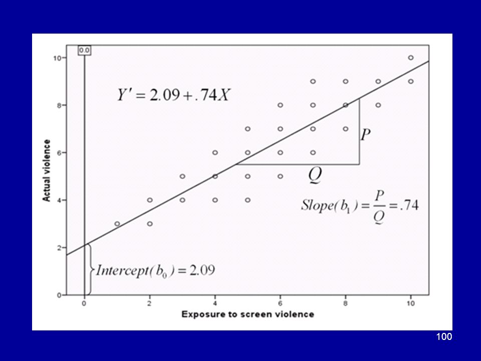
97. The regression line of Violence upon Preference
The REGRESSION LINE is the line that fits the points best from the point of view of predicting Actual Violence from Preference.
(A different line would be drawn were we to try to predict Preference from Actual Violence.)

99. Here is the equation of the regression line

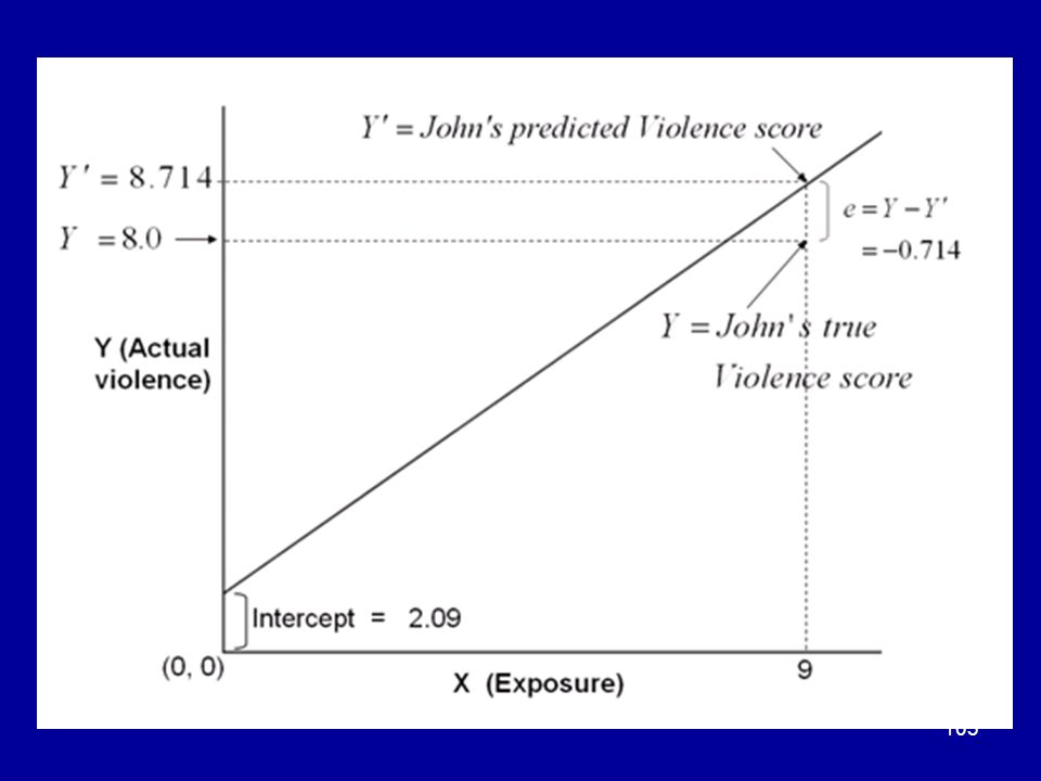
102. Residual scores
Suppose we use the regression line of Y upon X to predict the value of a person’s score Y from a particular value of X.
A RESIDUAL (e) is the difference between a person’s true score on Y and the point on the regression line.

104. The residuals are shown in the next picture

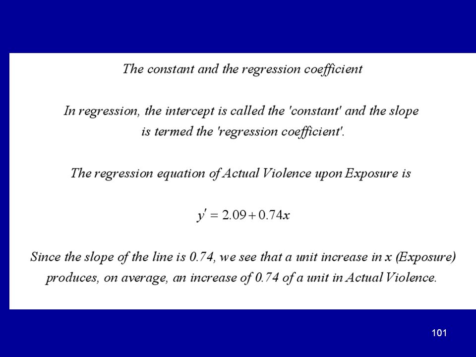
106. Summary B1 is the slope and B0 is the intercept.
Y/ is the Y-coordinate of the point on the line above the value X.
An increase of one unit on variable X will result in an estimated increase of (B1) units on variable Y.
A NEGATIVE value of B1 means that an increase of one unit on variable X will result in an estimated REDUCTION of B1 units on Y.
regression constant (intercept)
regression coefficient (slope)

107. The ‘least-squares’ criterion
The regression line is the ‘best-fitting’ line in the sense that it minimises the sum of the squares of the residuals.

109. Breakdown of the total sum of squares

110. Coefficient of determination

111. Explanation

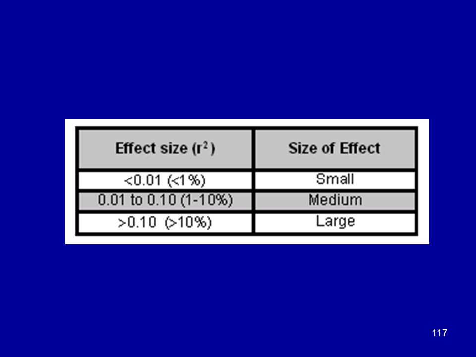
112. The coefficient of determination (r2)
The COEFFICIENT OF DETERMINATION (r2) is the proportion of the variance of the predicted variable accounted for by regression.
The coefficient of determination can take values within the range from 0 to +1, inclusive.

113. Range of r

115. Positive bias
The coefficient of determination is positively biased as an estimator.
The statistic known as ‘adjusted R2’ attempts to correct this bias.

118. Using more than one regressor
By analogous methods, we could try to predict a person’s actual violence from exposure to screen violence and number of years of education.
This is a problem in MULTIPLE REGRESSION.

119. Multiple regression

120. Geometrical interpretation
This is the equation of a plane (or hyperplane) with slopes B1, B2, …,Bp with respect to axes X1, X2, …, Xp and intercept B0.
The slopes are the PARTIAL REGRESSION COEFFICIENTS and the intercept is the CONSTANT.

121. Regression coefficients
In simple regression the REGRESSION COEFFICIENT (B1 ) is the estimated change in units of the DV that would result from an increase of one unit in the IV.
In multiple regression, a PARTIAL REGRESSION COEFFICIENT such as B1 is the estimated change in the DV resulting from an increase of one unit in the IV X1 with ALL OTHER IVs HELD CONSTANT.

122. The multiple correlation coefficient R
The MULTIPLE CORRELATION COEFFICIENT is the correlation between the estimates Y/ and the actual values of the DV (Y).
The COEFFICIENT OF DETERMINATION (R2) is the proportion of the variance of Y that is accounted for by regression.

123. Range of R
The multiple correlation coefficient R can only have non-negative values:
0 ≤ R ≤ +1
This is because the regression line (or plane) cannot have a slope of opposite sign to that of the elliptical (or hyperelliptical) scatterplot.

124. Attribution of variance to regressors
If the IVs are uncorrelated, it is easy to attribute variance in Y to each of the independent variables X.

126. Correlated IVs
When the IVs are measured, they always correlate to at least some extent.
It is then impossible to attribute variance unequivocally to any particular IV.

129. Dummy variables
Information about group membership is carried by a grouping variable.
A DUMMY VARIABLE has only two values: 0 and 1, where 0 usually denotes the control or comparison condition – in this case the Placebo.

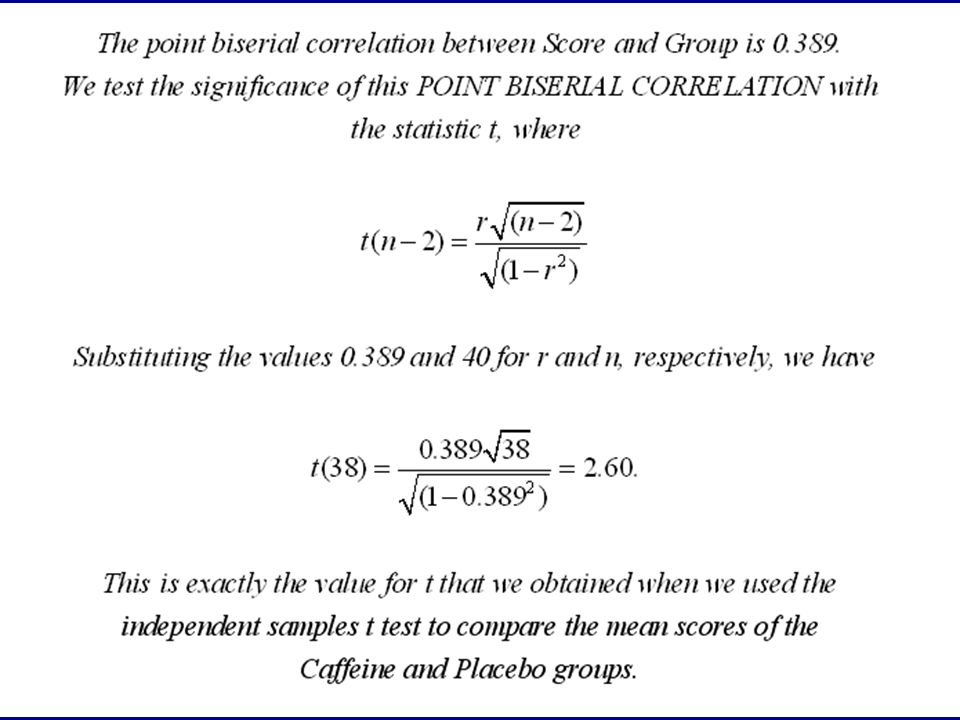
130. Point-biserial correlation
If we correlate the scores in the Group column with the dummy variable in the Score column, we obtain what is known as a POINT-BISERIAL CORRELATION.
The meaning of ‘point-biserial’ is lost in the mists of antiquity.
The point is that we are correlating a measured variable with code numbers for category membership.

132. A link
The point biserial correlation is of limited value as a descriptive statistic.
However, it forms a useful conceptual bridge between the statistics of comparison (t-test) and association (correlation).

133. Regression upon dummy variables
We shall now regress the scores that people achieved in the Caffeine experiment against those of the dummy variable carrying group membership.

134. The regression line will pass through the group means1 X

135. Why?
OLS regression minimises the sums of the squares of the residuals.
In either group of scores, the sum of the squared deviations about the mean is a minimum.

136. The sum of squares of deviations about the mean is a minimum

137. The regression statistics
When we regress the Score variable against the dummy variable, the intercept of the regression line is the mean score of the Placebo group.
The slope of the regression line is the difference between the means of the Caffeine and Placebo groups.

138. The regression statistics

141. Significance tests
The intercept (Constant) is 9.25, the value of the Placebo mean.
The slope is 2.65, which is – 9.25, the difference between the Caffeine and Placebo means.
t(38) = 2.604; p = This is exactly the result we obtained with the independent samples t test.

142. Equivalence of ANOVA and regression
When we test the slope of the regression line for significance, we are also testing the difference between the Caffeine and Placebo means for significance.
Since (in the 2-group case) the F and t tests are equivalent, the regression ANOVA table is identical with the one-way ANOVA table we obtained before.

143. Dummy coding for the k-group case
Since MSbetween has only four degrees of freedom, regression will predict the treatment means perfectly if the Score variable is regressed upon four dummy variables X1, X2, X3 and X4.
As with the two-group example, an interesting equivalence emerges.

144. Dummy coding for the k-group case

145. The one-way ANOVA statistics

146. The regression statistics
Same as the ANOVA value of F.
We see that B0 is the Placebo mean and B1, B2, B3 and B4 are the differences between the means for the 4 drug conditions and the Placebo mean.

147. In summary
When the scores in the five-group drug experiment are regressed upon 4 dummy variables,
The regression constant or intercept B0 is the Placebo mean.
The partial regression coefficients are the differences between the drug conditions and the Placebo mean.
The regression sum of squares is equal to the ANOVA between groups sum of squares.

148. In summary …
The t - tests of the regression coefficients are equivalent to the t-tests of the sums of squares associated with the four contrasts.

149. Eta squared
Returning to the one-way ANOVA, recall that eta squared (also known as the CORRELATION RATIO) is defined as the ratio of the between groups and within groups mean squares.
It’s theoretical range of variation is from zero (no differences among the means) to unity (no variance in the scores of any group, but different values in different groups).
In our example, η2 = .447

150. Eta squared revisited
If the scores from a k – group experiment are regressed upon k – 1 dummy variables, the square of the multiple correlation coefficient R is the proportion of variance of the scores accounted for by differences among the treatment means.
Eta squared is R2, which I think is why it is also termed the ‘correlation ratio’.

151. Formula for SSψ
We can think of a contrast sum of squares as the between treatments variability that is accounted for by a particular contrast.
The sums of squares for orthogonal contrasts add up to the ANOVA between groups sum of squares.

152. The contrast sum of squares revisited

153. Building bridges
In these two sessions, in addition to revising (and adding to) some material with which you are already familiar, I have tried to demonstrate some striking equivalences between techniques which many think of as having quite different contexts and purposes.

154. Assignment before noon on Wednesday 31st October.
Please complete the project and hand it in to Anne
before noon on Wednesday 31st October.
I shall return your answers (with comments) by
Wednesday 7th November.