1. MRes Course 2007-2008 LOGLINEAR MODELLING

2. Risk factors in the incidence of an antibody
A researcher has reason to believe that there may be a higher incidence of a potentially harmful antibody in patients whose tissue is of a particular ‘critical’ type.
In a study of 79 patients, the incidence of the antibody in patients of four different tissue types is recorded.

3. Two variables or attributes
In this study there are two variables:
Tissue Type;
Presence (or absence) of the antibody.
We are trying to ascertain whether there is an association between them.

4. Contingency tables
A CONTINGENCY TABLE is a CROSSTABULATION of a nominal data set showing the frequencies of observations in different combinations of the categories making up two QUALITATIVE variables or attributes.

5. Here is a contingency table showing counts of the presence or absence of an antibody in the four different patient groups.

8. Today’s topic
You are already familiar with the chi-square test for association between two qualitative variables or attributes.
Today, I shall be considering the investigation of associations among the variables in more complex frequency tables with THREE OR MORE variables or attributes.

9. An experiment on helping
Male and female interviewers asked male and female participants whether, in a certain situation, they would be prepared to help someone in a jam.

10. A complex frequency table
The results of the helping experiment can be summarised in a contingency table with THREE VARIABLES:
Interviewer’s sex;
Participant’s sex;
Help (Yes or No).

12. Scientific hypothesis
In the Tissue Type and Presence experiment, the SCIENTIFIC HYPOTHESIS is that there IS an association between the two attributes.

13. The null hypothesis
The NULL HYPOTHESIS (H0) is that there is NO association between Tissue Type and Presence: the two attributes are INDEPENDENT.
It is the NULL HYPOTHESIS of independence, not the scientific hypothesis, that is tested by the traditional chi-square test for association.
With just two attributes, the interpretation of the test result is clear: if the null hypothesis is falsified, we have shown the presence of an association between the two attributes.

14. The chi-square test with three attributes
With three or more attributes, the traditional chi-square test can easily be adapted to test the null hypothesis of total independence among the attributes.
A significant result confirms that there is an association among the variables.

15. Ambiguity
The mere presence of an association, however, does not tell us which of the several variables are involved.
Are just two of the three variables associated? Are all three variables involved in associations? Are female participants more helpful than male participants? (That implies that the attributes of Help and Paricipant’s sex are associated.)
A significant result for the chi-square test cannot answer such questions.

16. The traditional follow-up analysis
Following the initial test, associations between specific pairs of variables were investigated by COLLAPSING the frequency tables across unwanted variables, leaving the pair you were investigating.
The usual chi-square test for association between the two variables could then be made.

17. Are females more helpful?
I collapse the frequencies across the variable of Interviewer’s sex.
I test for an association between Help and Participant’s sex.
The result is significant.
I conclude that females are more helpful.
Unfortunately, this conclusion is FALSE!

18. Danger!
The strategy of collapsing across variables in complex frequency tables is fraught with danger.
You can collapse across unwanted variables, make a chi-square test for an association between two target variables and obtain a significant result.
There may actually be NO association between those variables!

20. Hidden variables
The practice of collapsing across some variables makes them ‘disappear’.
But the vanished variables (Interviewer’s Sex) can continue to affect the appearance of the two-way table.
As a result, the researcher can come to a false conclusion.

21. The opposite-sex dyadic hypothesis
The helping experiment was designed to test the OPPOSITE-SEX DYADIC HYPOTHESIS, which holds that we are more likely to offer help to someone of the opposite sex than to one of our own sex.
None of the three possible two-way interactions (Help × Participant, Help × Interviewer, Participant × Interviewer) captures this hypothesis.

22. A three-way interaction
No test of any two-way association can confirm the opposite-sex dyadic hypothesis.
The hypothesis implies a THREE-WAY ASSOCIATION or THREE-WAY INTERACTION among the three variables.
The traditional chi-square test cannot test such a hypothesis.

23. Loglinear modelling
Recent years have seen great advances in the analysis of complex contingency tables.
A LOGLINEAR MODEL is an equation which accounts for the cell frequencies.
Any cell frequency is stated to be the sum of several terms, each of which resembles those in an ANOVA model: There are MAIN EFFECT terms and there are INTERACTIONS.
From the model, the UNIQUE contribution of each effect to the cell frequencies can be seen and each effect can be tested for statistical significance.

24. Complex interactions
In loglinear modelling, even complex interactions can be included in the model and their unique contribution to the overall association among the variables can be safely determined.

25. Where we are going
I shall start with the traditional chi-square test for association between two attributes.
I shall then compare the ordinary chi-square test with a loglinear analysis of the same data.
I shall then demonstrate the superiority of the loglinear approach by analysing the three-way contingency table of the results of the gender and helping experiment.

26. Returning to the incidence of the antibody in different tissue groups ….

28. Expected frequencies
For each cell of the contingency table, the EXPECTED FREQUENCY (E) is calculated on the assumption that the variables of Tissue Type and Presence are INDEPENDENT.
The values of E are calculated on the basis of the NULL HYPOTHESIS.

29. Rationale of the test
The expected frequencies E are compared with the OBSERVED FREQUENCIES (O).
If the values of O are very different from the values of E, we have evidence against the null hypothesis of independence.
We infer that there is indeed an association.

30. The Pearson chi-square statistic

31. Finding the expected frequencies
The expected frequencies E are calculated using estimates of probability.
Their values are calculated from the MARGINAL TOTALS of the contingency table and the TOTAL NUMBER of observations in the whole table N.
Note that for fixed marginal totals and grand total, the cell frequencies can vary considerably.

34. An implicit multiplicative model
In the rule for the expected freqencies, estimates of probability are MULTIPLIED together.
Implicitly, we have applied a multiplicative INDEPENDENCE MODEL to the data.
If the independence model is a good fit, the values of E will be close to the values of O; it it isn’t, there may be large discrepancies.

36. Degrees of freedom
In physical science, the DEGREES OF FREEDOM of a system is the number of constraints you need to determine its state fully.
Viewing the marginal and grand totals of the contingency table as a system, you have 8 cell frequencies.
But you need only specify values for THREE of them to determine those of the others.

38. Rule for obtaining the df
If attributes A and B consist of a and b categories, respectively, the degrees of freedom df of the chi-square statistic are given by the formula:

40. One parameter
The chi-square distribution has ONE parameter, the degrees of freedom.
You cannot assign a probability to an obtained value of chi-square until you have specified the sampling distribution by assigning a value to the degrees of freedom (df ).

41. The target distribution
Our chi-square statistic has THREE degrees of freedom.
To make a significance test, we must refer this value to the distribution of chi-square on THREE degrees of freedom.

42. Suppose the null hypothesis is true, you run your experiment 10, 000 times and calculate chi-square from each data set. Through sampling error, you will occasionally obtain large values.

44. The p-value
The p-value of in the chi-square distribution on 3 degrees of freedom is …
This value is less than 0.05, but greater than 0.01.
We report the test result as follows:
“The chi-square test for association is significant beyond the 0.05 level: χ2(3) = 10.66; p = 0.01.”
So the result is significant beyond the 0.05 level but not beyond the 0.01 level.

45. The likelihood-ratio (LR) chi-square
There is another statistic, known as the LIKELIHOOD-RATIO (LR) CHI-SQUARE, which is also approximately distributed as true chi-square.
For a given data set, the two statistics have similar values.
Tests for significance usually lead to the same result.

48. Similar values
The value of the likelihood ratio (LR) chi-square (11.06) is close to the value of the Pearson chi-square (10.66).
The significance test with either statistic results in the same decision about the null hypothesis.
It is the LR chi-square statistic that is used in loglinear modelling because, as we shall see, it has a very important property that the Pearson chi-square lacks.

49. Measuring strength of association
The chi-square statistic is unsafisfactory as a measure of association, because its value reflects the size of the data set.
Statistics such as the PHI COEFFICIENT, CRAMER’S V and GOODMAN AND KRUSKAL’S LAMBDA provide measures of the strength of the association between the two attributes.
They are all available on SPSS.

50. A 2 × 2 contingency table

51. You are allowed to collapse across categories in a two-way contingency table.

53. 2 × 2 tables
With two by two tables, there is another useful measure of association based on a measure of likelihood known as the ODDS.

54. The odds
The ODDS is a measure of likelihood which, like PROBABILITY, arises in the context of an EXPERIMENT OF CHANCE, such as rolling a die or tossing a coin.
The ODDS in favour of an outcome is the number of ways in which the outcome could occur, divided by the number of ways in which it could fail to occur.

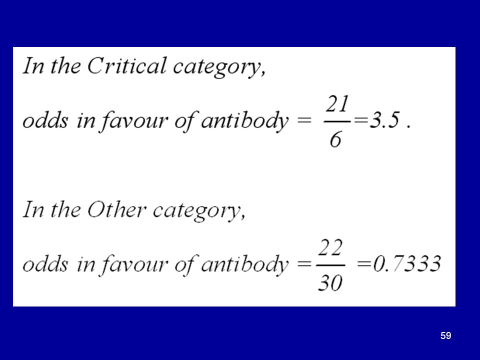
56. Example
Roll a die. There’s one way of getting a six; there are 5 ways of not getting a six.
The odds in favour of a six when a die is rolled are 1 to 5, or 1/5, to express it as a proper fraction.
Suppose we know that out of 100 people, 44 have a certain antibody in their blood.
The estimate of the ODDS in favour of a person having the antibody is 44 to 56 or 44/56.

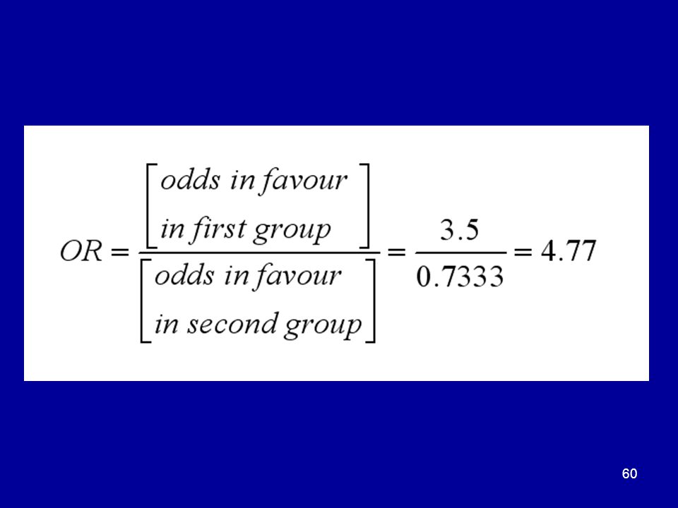
57. The odds ratio (OR)
We can compare the odds in favour of an outcome in TWO groups simply by dividing the two values.
This provides a useful measure of association known as the ODDS RATIO (OR).

61. Interpreting the OR
The odds in favour of the antibody in the Critical category are FIVE TIMES the odds in favour in the Other category. In other words, you are five times as likely to get the antibody in someone from the Critical group.
We shall see that the OR can be a valuable tool for exploring more complex contingency tables in which at least two of the attributes are DICHOTOMIES, that is, they each comprise only two categories.

62. The two-factor loglinear model
I am going to use SPSS to construct a loglinear model of the original 4 × 2 Tissue Type × Presence of Antibody contingency table.
The two-way loglinear model bears more than a superficial resemblance to the two-way fixed effects ANOVA model.

63. Revision of the model for the two-way ANOVA

64. A drug experiment
Here is a summary of the results of a drug experiment, in which the effects of two factors upon skilled task performance were studied.
The factors were Drug (Placebo, A, B) and Alertness (Fresh, Tired).

67. The interaction
The presence of an INTERACTION is suggested by the pattern of the CELL means.

69. The two-way ANOVA model
According to the two-way ANOVA model, the observed score X is made up in the following way:

71. Deviations
With the exception of the grand mean, the components of the ANOVA model are all DEVIATIONS, with the property that they sum to zero over all levels of either factor.
Although they are all calculated from the statistics of the sample, they are regarded as ESTIMATES of the corresponding population PARAMETERS.
The ANOVA model is expressed in terms of parameters, rather than sample statistics.

73. Model-building
EVERY statistical test is based upon a model, or interpretation of the data, which usually takes the form of an equation.
There is a model for every type of ANOVA.
But using the ANOVA is NOT a process of model-building as such.
The underlying model is retained regardless of the results of the ANOVA tests.

74. Loglinear modelling
Like the ANOVA model, a loglinear model interprets the data as the sum of a set of effects.
In model-building, however, terms are added or removed according to how well the model FITS the data.
A model might have many possible terms; but a much simpler model with very few terms might turn out to fit the data very well indeed.

75. The saturated model
A loglinear model that contains all possible terms is known as a SATURATED model.
The most complex term is so defined that a saturated model must predict the values of the cell frequencies (or their logs) PERFECTLY.
A saturated model has as many parameters as there are cells in the contingency table, leaving no degrees of freedom for any differences between the observed and expected frequencies.

76. The total degrees of freedom
The cells have 3 df.
The marginal row totals have 3 df.
The marginal column totals have 1df.
For a fixed N, there are a total of 7 degrees of freedom in this table.
The SATURATED MODEL has 7 degrees of freedom.

77. The saturated loglinear model
The saturated (or full) loglinear model of the cell frequencies in a two-way contingency table bears more than a superficial resemblance to the ANOVA model.
There is a grand mean, or CONSTANT.
There are MAIN EFFECT terms.
There is an INTERACTION term.

79. Note
We are effectively modelling the cell frequencies, not an individual score. There is NO RANDOM ERROR TERM in the loglinear model.
We are modelling, not the frequencies themselves, but their NATURAL LOGARITHMS.

80. Why logs?
We have seen that the expected frequencies are estimable from the marginal means by MULTIPLICATIVE, not SUMMATIVE rules. In fact, a multiplicative model of the expected cell frequencies is quite feasible.
The log of a PRODUCT is the SUM of the logs.
So if we model the LOG of the frequency, rather than the frequency itself, we shall have a SUMMATIVE, rather than a MULTIPLICATIVE, model.
This is the meaning of the term LOGLINEAR.

81. Parallels with the ANOVA model
The constant is the grand mean of the logs of the cell frequencies.
The main effects are the deviations of the logs of the marginal totals from the means of the logs of the marginal totals.
The interaction effect is what is left of the log of the cell frequency when the main effects have been removed.

82. Non-independence of marginal frequencies and effects
In the ANOVA, estimates of main effects and interactions are based upon MEANS.
The values of means are not dependent upon the numbers of observations from which the means have been calculated.
When we are modelling cell frequencies, however, the marginal frequencies do affect both main effect and interaction terms.

83. The hierarchical principle
When an interaction term is included in a loglinear model, the main effects of the factors involved must also be included.
When the interaction is complex (say three-way), all lower-order interactions among the factors must also be included in the model, as well as the main effects of the factors involved.

84. The generating class of a model
In most (though not all) SPSS procedures, you need specify only an interaction term: the procedure will follow the hierarchical principle and generate all lower order interactions (if there are any), as well as the main effect terms.
The GENERATING CLASS of a model is a list of all its distinct terms at highest level.
A model of generating class A, B×C×D, for example, will contain the main effect terms A, B, C and D, and the two-way interactions A×B, A×C and B×C, as well as the three-way interaction.

86. The main effects model
If the interaction is removed from the saturated model, we have an UNSATURATED MODEL known as the MAIN EFFECTS (or INDEPENDENCE) MODEL.
This, implicitly, is what is being tested by the traditional chi-square test.

88. The use of chi-square in loglinear modelling
We use the LR chi-square statistic as a measure of a model’s GOODNESS-OF-FIT.
If the model is a GOOD fit, the value of chi-square is SMALL and statistically insignificant.
If the model is a POOR fit, chi-square is LARGE and statistically significant.

89. Backward elimination strategy
Start with the saturated model. Chi-square has no degrees of freedom and a value of zero.
Remove the highest-order interaction. Chi-square will increase.
If chi-square increases significantly, the term must be retained in the model.
If the increase in chi-square is small and insignificant, the term can be dropped from the model.
The process continues until no term can be dropped without a significant increase in chi-square.

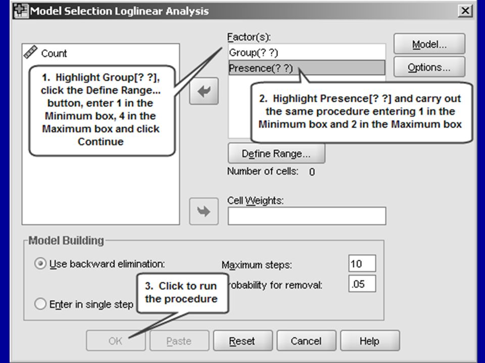
90. Using SPSS to model the Tissue Type × Presence contingency table

94. Use the table of output contents to find your way around.

101. The additive property
The advantage of the LR chi-square is that the total value for all effects can be partitioned into non-overlapping contributions from the different effects, so that the total value is the sum of the values associated with the separate effects.
You will see that the total Pearson chi-square is not quite equal to the sum of the chi-squares of the components.

102. Now, we’ll fit an unsaturated, main effects model
Now, we’ll fit an unsaturated, main effects model. Click the Model button.

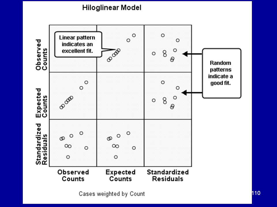
105. Graphing the residuals
A loglinear model is rather like a regression equation.
As in regression, the study of the residuals (O – E) affords insight into the goodness-of-fit of the model.
Difference kinds of residuals serve different purposes.
ADJUSTED and DEVIANCE residuals are good for identifying cells where the fit is poor.

109. Suppose the main effects model had been a good fit.

111. But this is how the graphs ACTUALLY appear!

113. Modelling a three-way contingency table

115. When attributes are dichotomies, the odds and odds ratios are useful tools for exploring a complex frequency table.

117. Interpretation of the odds ratios
For the males, OR = They were four times as likely to help if the interviewer was female than if the interviewer was male.
For the females, OR = They were twice as likely to help if the interviewer was male than if the interviewer was female.
There would appear to be some support for the opposite-sex dyadic hypothesis.

118. Effects in loglinear analysis and ANOVA
Suppose we had measured helpfulness on a continuous scale and analysed the data with ANOVA.
A main effect would have signified different levels of helpfulness.
A two-way interaction between Interviewer’s sex and Participant’s sex would have supported the opposite-sex dyadic hypothesis.

119. Interpreting effects in loglinear analysis
In our example, a main effect simply compares male and female interviewers and participants on frequency.
Main effects are often of trivial interest in loglinear analysis.
Differences in level of helpfulness emerge in TWO-WAY interactions. If female interviewers receive more help than male interviewers, there should be an interaction between Help and Interviewer’s Sex.
The opposite-sex dyadic hypothesis predicts a THREE-WAY interaction involving all three attributes: Help, Participant and Interviewer.

123. Notice that the two-way Participant
Notice that the two-way Participant*Help interaction does not make a significant contribution! It is only retained in the model in accordance with the hierarchical principle

125. Extension of the traditional chi-square test
The rule for obtaining the expected frequencies from elementary probability theory can be extended to complex contingency tables with three or more attributes.
A three-way contingency table can be presented as two two-way tables, each at a different LAYER of the third attribute.
Let R, C and L be the marginal total frequencies for the three attributes for one particular cell of the three-way classification.

130. Equivalence of chi-square test and total independence model
When we apply an extension of the traditional chi-square test to a three-way contingency table, we are effectively testing the goodness-of-fit of the main effects or total independence model.
But a significant result doesn’t confirm any specific association.
It could be one or more two-way interactions. It could be the three-way interaction. There could be interactions at both levels.
Our loglinear analysis has shown that the ONLY SIGNIFICANT TERM IN THE MODEL IS THE THREE-WAY INTERACTION.

131. Summary
The traditional chi-square test of independence can be extended to more complex frequency tables.
The rejection of the total independence hypothesis does not answer our research questions.
The traditional collapsing approach is dangerous; nor does it always answer the research question.
Loglinear modelling enables us to pinpoint the real associations and to test complex hypotheses that the traditional approach cannot test.

132. Further reading

133. Practical advice Kinnear, P. R., & Gray, C. D. (2007).
SPSS 15 Made Simple
Hove and new York: Psychology Press.
Chapter 13 outlines the rationale of loglinear modelling and gives you step-by-step instructions on how to run the procedure.

134. An excellent textbook
Howell, D. C. (2007). Statistical methods for psychology (6th ed.). Belmont, CA: Thomson/Wadsworth.
There’s a helpful introduction to loglinear modelling in Chapter 17.

135. Tabachnik, B. G. , & Fidell, L. S. (2007)
Tabachnik, B. G., & Fidell, L. S. (2007). Using multivariate statistics (5th ed.). Boston: Allyn & Bacon. Chapter 16.
Field, A. (2005). Discovering statistics using SPSS for Windows: Advanced techniques for the beginner (2nd ed.). London: Sage. Chapter 16.

136. Appendix Logarithms

137. A logarithmic system
In a LOGARITHMIC SYSTEM, numbers are expressed as POWERS of a constant known as the BASE.
The numbers 10, 100, 1000, 10,000,
100,000 and 1,000,000 can all be expressed as powers of 10 thus:

139. Definition of a log
The log of a number is the power to which the base must be raised to equal the number.
So, since 1000 = 103, the log of 1000 to the base 10 is 3.
The two most common bases are 10 and the number e, where e ≈ 2.72
Logs to the base e are known as NATURAL LOGS.

141. Notation for logs

142. Domain of the log function
The log of a negative number is not defined.
The log of zero is minus infinity.

143. Noteworthy logs The log (or ln) of 1 is zero because e0 = 100 = 1.
Ln (e) = Log (10) = 1
because eln(E) = e; 10log(10) = 10.

144. The antilog

145. The exponential function

146. Writing a number as an antilog
Any non-negative number can be written as an antilog: e.g.
y = exp[ln(y)] or eln y = 10log y
There is no log of zero; but the antilog of zero is 1.

147. The laws of logs
The definition of the antilog is the key to the derivation of the LAWS OF LOGARITHMS.
For example, the log of the PRODUCT is the SUM of the logs.

149. Three laws of logs The log of the PRODUCT is the SUM of the logs.
The log of the QUOTIENT is the DIFFERENCE between the logs.
The log of the POWER is the power TIMES the log.

150. Things to remember about logs
There is no log for a negative number.
The log of zero is minus infinity.
A log can have a negative value. It does so when the number is a PROPER FRACTION (numerator less than the denominator, so with a value between zero and 1).
The log of 1 is zero.