1. SESSION 2 FACTORIAL ANOVA AND RELATED TOPICS

2. The one-way ANOVA In Monday’s session, I revised the one-way ANOVA.
We saw that merely obtaining a significant F and therefore rejecting the null hypothesis of equality of the means was just the first step.
Before leaving the one-way ANOVA, we must look at some more of the techniques that are used in the follow-up analysis.

3. Does SIGNIFICANT mean SUBSTANTIAL?
The F test produced a significant result.
The null hypothesis of equality of the five treatment means must be rejected.
With large numbers of observations, however, a statistical test can have too much POWER to reject the null hypothesis, that is, even tiny differences among the means will result in a significant F.
‘Significant’ does not necessarily mean ‘substantial’.

4. Partition of the total sum of squares

5. Eta squared
The oldest measure of effect size is suggested by the partition of the total sum of squares.
In this measure, the between groups sum of squares is expressed as a PROPORTION of the total sum of squares.
The greater the proportion of the total sum of squares that is accounted for by the between groups sum of squares, the greater should be the spread among the means in the population.

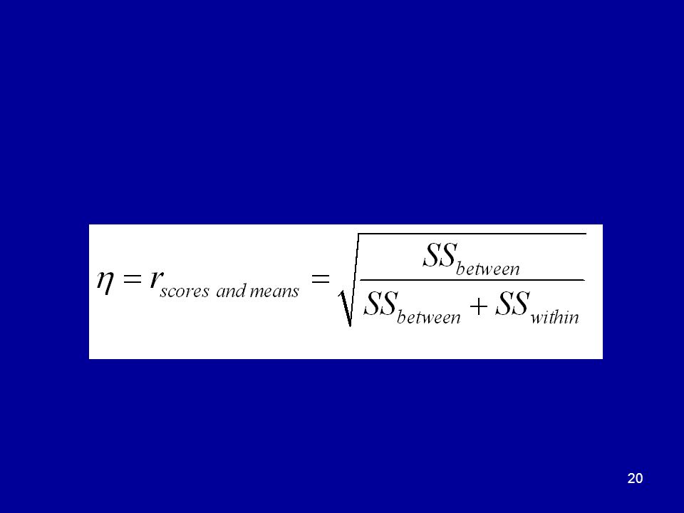
6. Eta squared (where eta is the CORRELATION RATIO)

7. Maximum value of eta squared
If there were differences among the treatment means and NO ERROR VARIANCE AT ALL (everyone in each group got the same score), the value of eta squared would be 1.

8. Minimum value
If there were no differences among the means, the between groups sum of squares would be zero and so would the value of eta squared.

9. Range of eta squared
Theoretically, therefore, eta squared can take values between zero and (plus) one.
In practice, its values will lie somewhere between these limits.

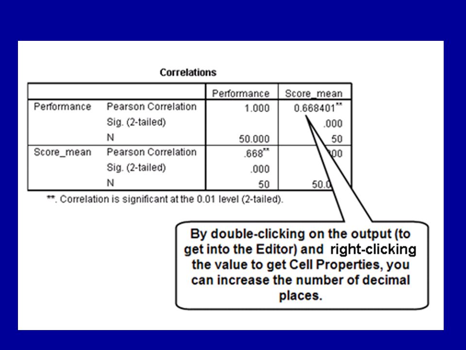
10. Why is eta called the ‘correlation ratio’?
Suppose that opposite each of the 50 scores in the one-way drug experiment, we were to place the value of the mean of the participant group in which the score was achieved.
The correlation between the column of scores and the column of means gives the value of eta.
Let’s demonstrate this.

11. Use the Aggregate command

12. The Aggregate procedure
In SPSS, the Aggregate procedure places opposite each score a value (such as the mean – but other statistics can be chosen) which summarises the scores in the group.
The group is specified as the BREAK VARIABLE.
The participant’s score (the DV) is the VARIABLE TO BE SUMMARISED.

14. The column of means has been created

15. Now correlate the means with the scores …

19. The square of the correlation between the scores and the group means is eta squared. Eta is the correlation between the group means and the scores.

21. What eta squared is supposed to be measuring in the population

22. Positive bias
Eta squared is positively biased as an estimate of effect size.
Were the experiment to be repeated many times, the long run average or EXPECTED VALUE of eta squared would be higher than the population value.

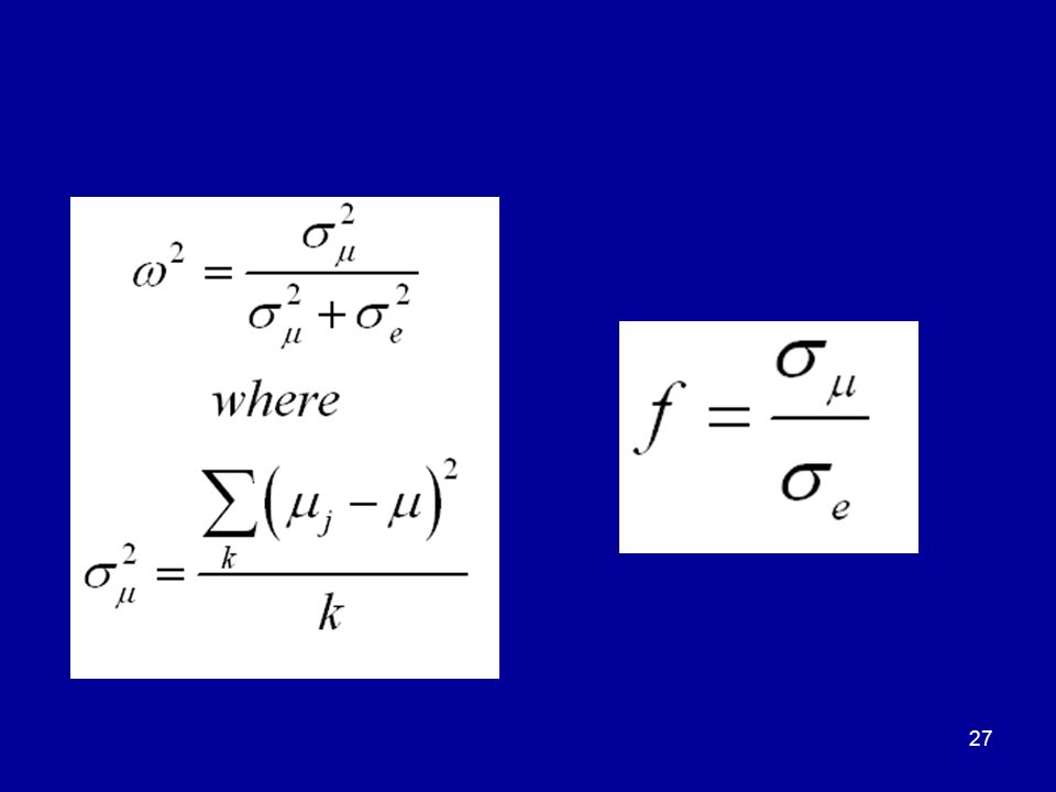
23. Omega squared
Omega squared is another measure of effect size, intended to be an unbiased estimate of the following:

24. This estimate of omega squared tries to overcome the positive bias in eta squared

25. G*Power
There is an excellent package, available free on the Internet, which can answer many important questions about power and sample size.
You must explore this package and get to know how to use it.
To use G*Power, you must express your questions in terms of another measure of effect size, known as Cohen’s f.

26. Cohen’s f

29. Equivalent values
We have found that the estimate of omega squared from our data is 0.39.
Applying the equivalence formula, we find that

30. Which measure? SPSS provides only the eta squared measure.
A journal editor might ask you to provide an estimate of omega squared or f.
On the other hand, there are experimental designs for which it is difficult to produce unbiased estimates of omega squared and f. In such situations, we must make do with eta squared.

31. Using the table
If you have only a value of eta squared, compare it with the values in the omega squared column of the table. Your reader, however, may expect you to convert your eta squared to the equivalent value of omega squared.

32. Multiple comparisons
When there are three or more groups, the rejection of the null hypothesis leaves many important questions unanswered, such as the location of robust differences among the individual treatment means.
On Monday, I discussed the making of specific PRE-PLANNED comparisons, simple and complex, among the individual treatment means.

33. Two-group t test

34. k-group t statistic for multiple pairwise comparisons

35. More power
If you use the error term for the whole design, rather than one calculated from the two groups concerned, your test will be more powerful.
When the degrees of freedom of the error term are increased, a lower value of t will achieve signficance.

36. Type I errors
Returning to the two-group experiment and the independent samples t test, if the sigificance level α is set at 0.05, any p-value less than 0.05 will result in the rejection of the null hypothesis.
If the null hypothesis is true, it will be wrongly rejected on 5% of occasions with repeated sampling. A false rejection of the null hypothesis is known as a ‘Type I’ error, and the significance level is therefore also known as the ‘Type I’ or ‘alpha’ error rate.

37. The per comparison and familywise Type I error rates
Returning to ANOVA and our array of k treatments means, suppose that we plan to make a set of c comparisons among a set of means.
If the alpha or significance level is set at 0.05, the Type I error rate PER COMPARISON is 0.05.
But what is the probability that AT LEAST ONE COMPARISON will show significance, even when the null hypothesis is true?
This probability is known as the FAMILYWISE Type I error rate.

38. Capitalising upon chance
With a large array of treatment means, we might decide to make a large number of comparisons.
Even if the null hypothesis is true, the familywise Type I error rate might be 0.90 or even higher!
Failure to take the heightened probability of a Type I error into account when making sets of comparisons is known as CAPITALISING UPON CHANCE.

39. The Bonferroni formula
If alpha is the significance level for each comparison, it can be shown that the familywise Type I error rate is approximately c times alpha, where alpha is the usual significance level.
Let’s call this the BONFERRONI FORMULA, from a related theorem in probability theory.

40. Conservative tests
A CONSERVATIVE TEST adjusts the p-value per comparison upwards in order to to control the familywise Type I error rate.
This is equivalent to setting the per comparison significance level at a lower value than the traditional significance level.
There are many different approaches to the making of conservative tests to avoid capitalising upon chance.

41. The Bonferroni correction
The Bonferroni formula suggests how a conservative test might be made.
Simply multiply the p-value of each comparison by c and reject the null hypothesis only if the adjusted p-value is smaller than the intended FAMILYWISE significance level, which is usually set at 0.05.
Alternatively, set the per comparison significance level at 0.05/c, where c is the number of comparisons you intend to make.

42. The Bonferroni correction

43. Application to contrast sets
The Bonferroni correction was first applied to sets of planned comparisons such as Helmert contrasts or simple contrasts.
If you plan to make c contrasts, just divide the traditional significance level (0.05) by c.
So if you plan to make 4 contrasts, you would require a p-value of less than 0.05/4 =0.01, approximately, before declaring a comparison significant.

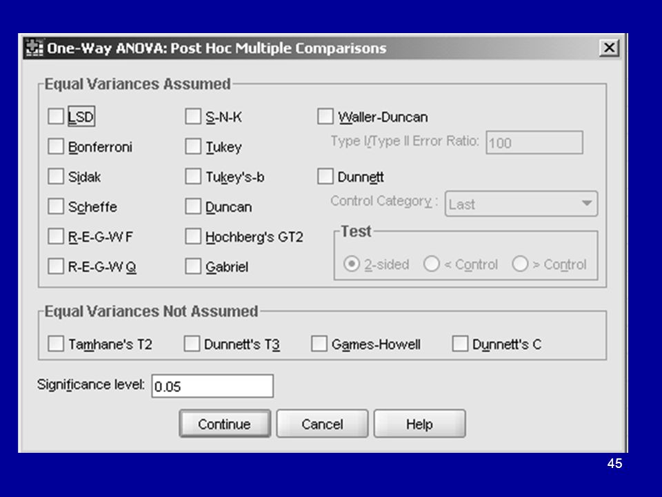
44. Unplanned or ‘post hoc’ comparisons
Often, the researcher isn’t in a position to plan a specific set of comparisons before the data have been gathered.
More usually, once the data have been gathered, the initial ANOVA is followed by an a posteriori process of data-snooping, which involves the making of unplanned or POST HOC comparisons.
Many post hoc tests have been proposed.

46. Which one?
The Bonferroni is the most conservative of these tests. With a large array of means it’s almost impossible to get anything significant.
In between subjects experiments, the Tukey test is preferred.
The Dunnet is the most powerful test, but suitable only for the situation where you are comparing the mean of the controls with each of the other treatment means, that is, when you are making simple comparisons.

47. Factorial experiments
In a FACTORIAL experiment, there are two or more treatment factors.
The ANOVA really comes into its own when it is applied to the analysis of data from factorial experiments.

48. Types of ANOVA design The three most common types of ANOVA design are:
BETWEEN SUBJECTS FACTORIAL designs, in which ALL factors are between subjects.
WITHIN SUBJECTS FACTORIAL designs, in which ALL factors are within subjects.
MIXED FACTORIAL designs, in which SOME factors are between subjects and some are within subjects.

49. An experiment with two treatment factors
Suppose that a researcher has been commissioned to investigate the effects upon simulated driving performance of two new anti-hay fever drugs, A and B. It is suspected that at least one of the drugs may have different effects upon fresh and tired drivers, and the firm developing the drugs needs to ensure that neither drug has an adverse effect upon driving performance.
The researcher decides to carry out a two-factor factorial experiment, in which the factors are:
Drug Treatment, with levels Placebo, Drug A and Drug B;
Alertness, with levels Fresh and Tired.

52. Main effects and interactions
A factor is said to have a MAIN EFFECT if, in the population, there are differences among the means at its different levels, ignoring any other factors there may be in the design.
In factorial experiments, interest usually centres not on main effects, but on the interplay among the treament factors, that is, upon INTERACTIONS.

53. Observations Main effects are evident in the MARGINAL TOTALS.
Not surprisingly the Fresh participants outperformed the Tired participants.
Performance was higher in the Drug B group.
But the cell means are the main focus of interest, because certain patterns indicate the presence of an INTERACTION.
A PROFILE PLOT is of great assistance in interpreting cell means.

54. Profile plots
Profile plots are the best way of determining whether any interactions are present and the precise nature of any interactions there may be.
More than one plot is possible: your choice depends upon which factor is of principal interest.

55. Two body state profiles

56. Three drug profiles

57. An interaction In neither plot are the profiles parallel.
In the first profile, the factor of Body State seems to reverse its effect at different levels of the Drug factor.
In the second profile, the ordering of the means at the three levels of the Drug factor changes from level to level of the Body State factor.
When one factor does not have the same effect at all levels of another, the two factors are said to INTERACT.

58. In summary …
If the profiles are parallel, there may be main effects, but there is no interaction.
Main effects are indicated by separation of the profiles and slope.
NON-PARALLELISM of the profiles indicates the presence of an interaction.

59. Partition of the sum of squares in the two-factor (two-way) ANOVA

60. Partition in the two-way ANOVA

61. Three F tests

62. Two-way ANOVA summary table

63. Effect size in factorial experiments
A controversial area.
The measure known as COMPLETE ETA SQUARED expresses the contribution of a source (whether a main effect or an interaction) to the total variance in the presence of all other treatment or group sources.
The measure known as PARTIAL ETA SQUARED excludes all other treatment or group sources.

64. Complete eta squared for Alertness

65. Partial eta squared for Alertness

66. Estimate of partial omega squared

67. Simple effects
The main effect of one factor at ONE LEVEL of another is known as a SIMPLE MAIN EFFECT.
If an interaction is significant, it is common practice to ‘unpack’ it by testing for the presence of simple main effects.

69. Simple main effects of Body State

70. Simple main effects of Drug

71. Testing for a simple effect

72. Simple effects with SPSS
Simple effects are not an option in the ANOVA dialog windows.
It is easy to run simple effects on SPSS, but we must use SYNTAX to achieve this.
A small problem is that we must use, not the ANOVA syntax command, but the command for what is known as Multivariate Analysis of Variance or MANOVA.

73. Multivariate analysis of variance (MANOVA)
In the ANOVA, there is just ONE dependent variable.
Multivariate Analysis of Variance (MANOVA) is a generalisation of the ANOVA to the analysis of data from experiments of ANOVA design with two or more DVs.
We can, therefore, regard the ANOVA as a special case of the MANOVA.

74. Using MANOVA to run ANOVA
If there is only one DV, running the MANOVA procedure will run a univariate ANOVA and produce the usual ANOVA summary table.

75. The basic MANOVA command

76. Get into the syntax editor…

77. Run the procedure

78. You get exactly the same ANOVA summary table as before.

79. The /ERROR and /DESIGN subcommands for simple effects of Drug

80. Output for simple effects analysis

81. The need for multiple comparisons

82. The need for a smaller comparison ‘family’
An interaction is significant.
We want to make unplanned or post hoc multiple comparisons among the treatment means.
But there may be many cells in the design, so that the critical difference for significance may be impossibly large.
In terms of the Bonferroni test, you could be multiplying the p-value by a large factor or setting the per comparison significance level at a tiny value.
We need to justify making the comparisons among a smaller array of means.

83. First, we test for simple main effects
We might argue that if we have a significant main effect of the Drug factor at one level of Body State or Alertness, we can define the comparison family in relation to those means at the Fresh level of Body State only. This will produce a less conservative test.
When testing for simple main effects, however, we should use the Bonferroni correction to control the familywise Type I error rate.
In our example, since there are two simple main effects, the criterion for significance should be that p is less than 0.025, rather than 0.05.

84. Reduce the data set.
There is more than one way of making the multiple comparisons.
You can easily run a one-way ANOVA on the data from the scores of the fresh participants only, then ask for a Tukey test.

85. Select the data from the Fresh participants only

86. Choose Tukey multiple comparisons

87. The results

88. Summary
A report of an ANOVA F test should be accompanied by a measure of effect size, such as eta squared or (preferably) omega squared. Follow Lisa DeBruine’s guidelines.
Beware of capitalising upon chance: follow-up tests should be conservative.
When unpacking significant interactions, use syntax to test for simple main effects.
A significant simple main effect can be an argument for a smaller comparison ‘family’.

89. Recommended reading
For a thorough and readable coverage of elementary (and not so elementary) statistics, I recommend …
Howell, D. C. (2007). Statistical methods for psychology (6th ed.). Belmont, CA: Thomson/Wadsworth.

90. For SPSS May I immodestly suggest …
Kinnear, P. R., & Gray, C. D. (2008). SPSS 16 for windows made simple. Hove and New York: Psychology Press.
In addition to practical advice about using SPSS 16, we also offer informal explanations of many of the techniques.