1. Logistic regression

2. Regression
Regression is a set of techniques for exploiting the presence of statistical associations among variables to make predictions of values of one variable (the DV, TARGET or CRITERION) from knowledge of the values of other variables (the IVs or REGRESSORS).

3. Simple and multiple regression
In SIMPLE regression, there is just one IV.
In MULTIPLE regression, there are two or more IVs.
In simple regression, a REGRESSION LINE is drawn through the points in the scatterplot.

5. General form of the simple regression equation

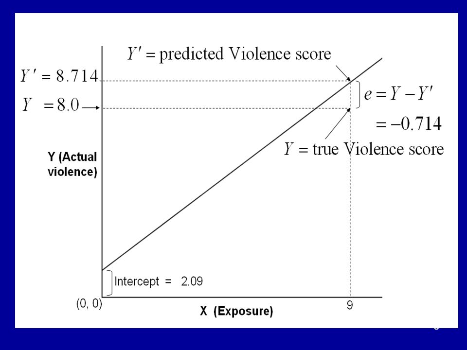
6. Estimates
The points on the regression line serve as ESTIMATES of the target variable or DV Y from the values of the IV X.

7. Residuals
We can make a good estimate of John’s score on Actual violence from a knowledge of the regression line and his score on Exposure.
But such estimation is subject to ERROR.
The error in our estimate is known as a RESIDUAL.

9. Goodness-of-fit: The LEAST-SQUARES criterion

11. Ordinary least-squares (OLS) regression
This approach to regression is known as ORDINARY LEAST SQUARES (OLS) regression.
There are other kinds of regression (such as LOGISTIC REGRESSION, today’s topic) which do not work in this way.

12. Coefficient of determination

13. Using more than one IV
We could try to predict a person’s actual violence not only from exposure to screen violence, but also from additional variables, such as number of years of education and characteristics of the parents.
These are problems in MULTIPLE REGRESSION.

14. Multiple regression

15. Partial regression coefficients
In multiple regression, a PARTIAL REGRESSION COEFFICIENT is the estimated average change in the DV resulting from an increase of one unit in one particular IV with ALL THE OTHER IVs HELD CONSTANT.

17. Coefficient of determination
In multiple regression, the COEFFICIENT OF DETERMINATION is the square of the multiple correlation coefficient.

19. What if the DV is a set of categories?
Simple and multiple OLS regression assume that the DV and IVs consist of measures on an independent scale with units. The term CONTINUOUS VARIABLE is used for this sort of DV.
But suppose we want to predict whether a person will suffer from a heart attack or contract a certain illness with known risk factors.
Here, we are not predicting a VALUE, but membership of a CATEGORY.

20. Category prediction: the OLS approach
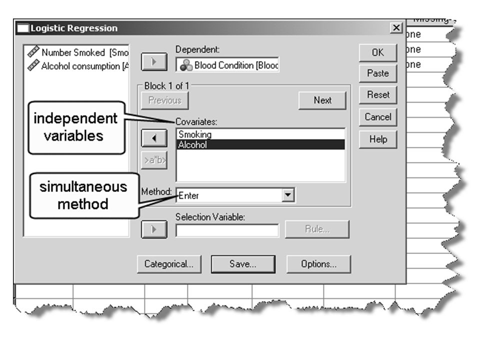
You are trying to predict the presence or absence of a blood condition, which is thought to be made more likely by smoking and alcohol consumption
Why not let 0 = Condition Absent; let 1 = Condition Present and calculate the usual OLS multiple regression equation?

21. Problems
There are serious problems with OLS regression when the DV is a set of categories.
None of the proposed solutions is entirely satisfactory.
There are better approaches.

22. Techniques for regression with a categorical DV and continuous IVs
The 2 most commonly used techniques are:
Discriminant analysis
Logistic regression

23. Discriminant analysis
If all (or most) IVs are continuous, you can use DISCRIMINANT ANALYSIS (DA).
But the DA model makes assumptions about the distributions of the IVs which data sets often fail to satisfy.

24. Logistic regression
Logistic regression makes fewer assumptions than discriminant analysis.
Logistic regression, moreover, is happy with CATEGORICAL IVs.

25. Logistic regression…
It is suspected that smoking and drinking are risk factors in the incidence of a pre-morbid blood condition, characterised by the presence of an antibody.
Records of the incidence of the condition in 100 patients are available, together with estimates of the amount they smoke and drink.

26. A section of the data

27. How many have the condition?

28. Forty-four patients have the condition

29. Back to OLS regression again
CONSTANT = MY – b1 MX
If X and Y are independent, the regression line will be close to horizontal (b1 = 0).
You might as well just guess the value of Y as MY every time, whatever the value of X.

30. Regression line with independence
When the variables show no association, the slope of the regression line is zero and the line runs horizontally through the mean MY of the criterion or dependent variable.

31. Intercept-only prediction
Whatever the degree of association between X and Y, the INTERCEPT- ONLY prediction is

32. Building regression models
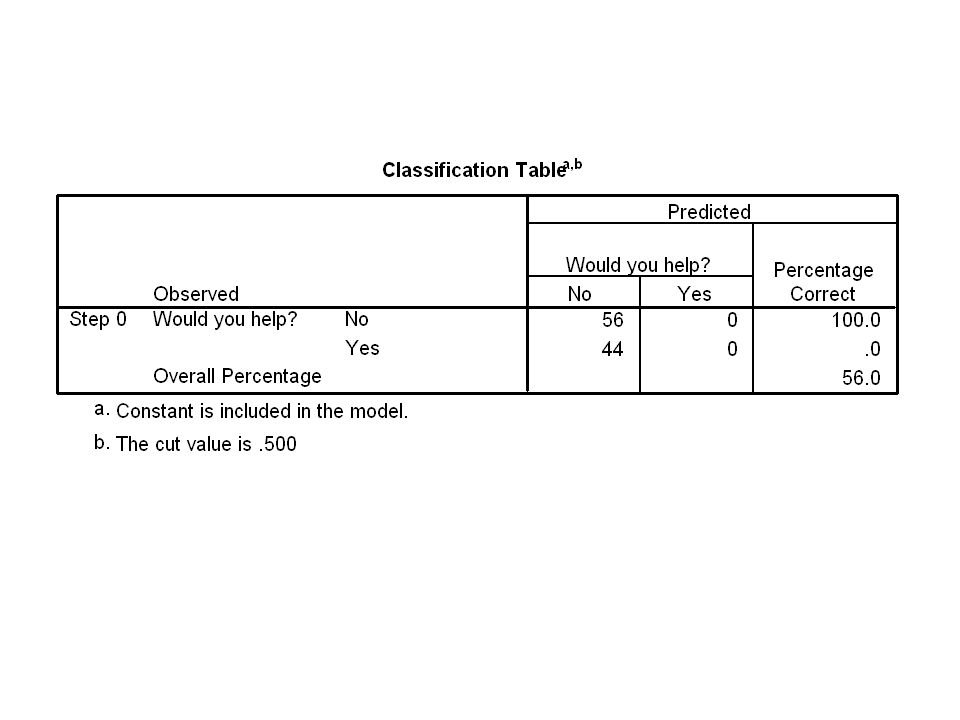
In model-building, we use the intercept-only (no regression) model as a BASELINE to assess the relative ability of the regression model to explain the variance of Y.
In our current example, the equivalent prediction is that, since 44/100 people have the condition, an individual will NOT have the condition.

33. Guessing: the no-regression success rate
If we decide to predict absence for every case, we shall be correct 56/100 times.
This is the equivalent of INTERCEPT-ONLY prediction in linear regression.

34. Assumption Either you have the disease or you don’t.
As smoking and alcohol increase, however, we assume that the probability of developing the condition increases CONTINUOUSLY as a function of the IVs.
In logistic regression, we estimate the probability of the condition with the LOGISTIC REGRESSION FUNCTION
Once the estimated probability exceeds a cut-off (usually .5), the case is classified as a Yes, rather than a No.

35. A logistic regression function

36. The decision rule
If the predicted probability is .5 or higher, assign to the condition-present category.

37. The odds
In an EXPERIMENT OF CHANCE (tossing a coin, rolling a die) the ODDS in favour of an event is the number of ways in which the event could occur, divided by the number of ways in which it could fail to occur.

38. The odds …
Roll a die. There’s one way of getting a six; there are 5 ways of not getting a six.
The odds in favour of a six when a die is rolled are 1 to 5.
Suppose we know that out of 100 people, 44 have a certain antibody in their blood.
The ODDS in favour of a person having the antibody are 44 to 56 or 44/56.

39. The log odds (logit) The odds measure suffers from ASYMMETRY OF RANGE.
Unlikely events have odds between 0 and 1; likely events can have huge odds.
The LOG ODDS (LOGIT) is the natural logarithm of the odds.
Logit = ln(odds) = loge(odds).

40. When the logit is zero Suppose the odds are 50 to 50 (50/50 =1).
Since the log of 1 is zero, a logit of zero means that the odds for are equal to the odds against.

41. Range of the logit
The logit has a symmetrical range: a positive sign means the odds are in favour; a negative sign means the odds are against.
The logit has no upper or lower limit: it has an unlimited range of values.

42. Example
The odds in favour of a case having the antibody are 44/56 = 11/14.
Logit = ln(11/14) = –.24
The event is less likely than not.
If the odds in favour were 56/44, the logit would be ln(56/44) = +.24.

43. Probability
A probability is a measure of likelihood ranging from 0 (an impossibility) to 1 (a certainty).
The probability p of an event is the number of ways it can happen divided by the total number of outcomes.
The probability of a six when a die is rolled is 1/6.

44. Relationship between p and odds
A probability and the odds are both measures of likelihood.
They are related according to the equation on the left.

45. Antilogs
We can write any positive number as an ANTILOG, that is, as the BASE raised to the power of the LOG of the number to that base.

46. The antilog

47. The odds as an antilog

48. The probability and the logit

49. The logit equation

50. The logistic regression equation

51. The problem
In the logit equation, we must find values for the intercept and the regression coefficients such that the accuracy of assignments of cases to categories is maximised.

52. No mathematical solution
In logistic regression, there is no equivalent of the formulae for the intercept and coefficients in OLS regression.
A ‘brute force’ computing algorithm is used in the hope that estimates of the coefficients will ‘converge’ to stable values.
We must check this ‘convergence’ by examining the ITERATION HISTORY in the SPSS output.

53. Potential difficulties
The algorithm will not run successfully if the IVs are too highly correlated. This is the familiar MULTICOLLINEARITY PROBLEM we encountered in OLS regression.
As with any multiple regression, it can be difficult to attribute the DV (category membership in this case) unequivocally to any one DV.

54. The meaning of a logistic regression coefficient
The regression coefficient is the increase in the logit in favour of an individual having the condition produced by an increment of one unit in the IV.
Suppose that for Smoking, b = An increase of one smoking unit (eg 10 cigarettes) increases the logit (the log odds) by 1.1.

55. Regression coefficients …
In terms of the ODDS, an increase of one unit in the IV MULTIPLIES the original odds by the ANTILOG of b, that is, by eb, or exp(b).
Exp(1.1) = 3.0
So an increase of one smoking unit results in the odds being MULTIPLIED by 3, that is, the event is three times as likely to happen.

56. Correlations

57. Observations
There’s a substantial correlation between one of the IVs and the DV. Good.
There’s little association between the IVs. Very good.
It looks good for the regression procedure.

58. Finding logistic regression

62. ‘Intercept-only’ hit rate.
‘Intercept-only’ estimation

63. Iteration
The logistic regression procedure chooses values for the coefficients such that the logistic regression function maximises correct category assignment.
But (unlike the situation in multiple regression) there is no mathematical solution to this problem: the procedure follows an algorithm which continuously works out estimates until these ‘converge’ on the set of values eventually used.

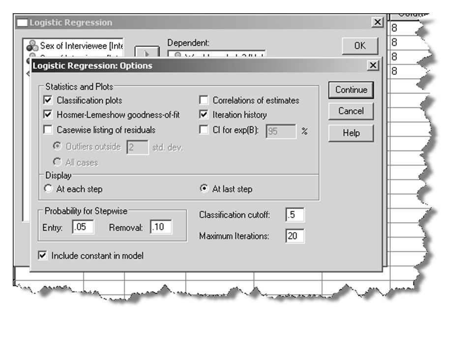
64. Iteration…
You need to check that the procedure produced estimates that did indeed converge.
You should ask for an ITERATION HISTORY to confirm that convergence took place.

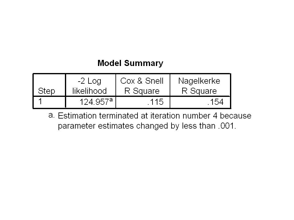
66. The Nagelkerke R2 statistic
The Nagelkerke statistic is the counterpart of the coefficient of determination R2 in OLS multiple regression.
It is a measure of the proportion of the total variation in incidence of the blood condition accounted for by regression.

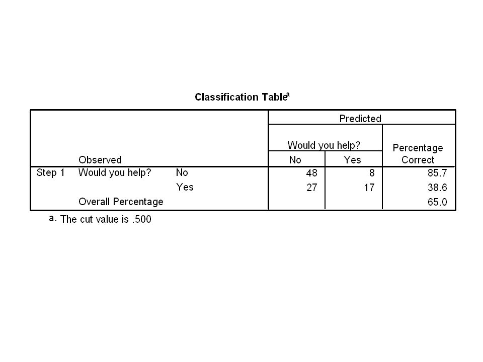
70. A regression model is now applied.
Hit rate using the regression model. This is obviously much better than the ‘intercept-only’ hit rate of 56%.
A regression model is now applied.

71. This is the antilog of the coefficient of Smoking in the logit equation. Increasing Smoking by one unit MULTIPLIES the odds in favour of occurrence by about 10.

75. Summary
The incidence of the blood condition is indeed predictable from regression and raises the hit rate from 54% to 85%.
Smoking contributes significantly to the model.
Alcohol does not contribute significantly to the model.

76. An example with categorical IVs
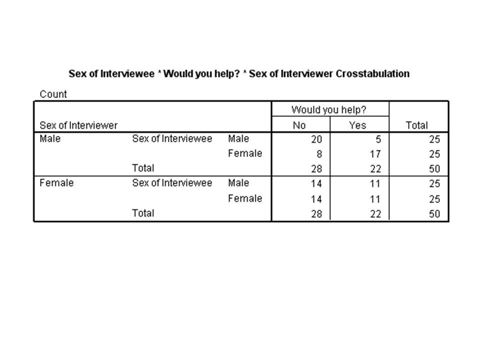
An experiment on helpfulness.
Do people tend to be more helpful to those of the opposite sex? This is the OPPOSITE-SEX DYADIC HYPOTHESIS.
Male and female interviewers asked male and female participants whether they would help in a hypothetical situation.

79. Interviewer’s sex
Helped? No Yes

80. Interpretation of ORs
When the interviewer is female, the OR is .118; but when the interviewer is male, the OR is 1.
This asymmetrical pattern only partially confirms the opposite-sex dyadic hypothesis.
But it seems that an interaction is present.

83. Complete the dialog

87. An interaction pattern

100. The only significant result is an interaction between Sex of Interviewer and Sex of Interviewee.

102. Conclusion
The OPPOSITE-SEX DYADIC HYPOTHESIS receives some support from this study.
Both sexes, however, tended to be on the unhelpful side with female interviewers.

103. A loglinear analysis
Since we have categorical variables, we can apply a loglinear analysis to the same data.
We can expect a similar result.

107. This p-value is similar to the value
This p-value is similar to the value .014 that we obtained with logistic regression.
This is the row reporting the results of a test for an interaction between Sex of Interviewer and Sex of Interviewee. It is the only significant effect.

108. Conclusion
The loglinear analysis leads to exactly the same conclusion as the logistic regression.
Both techniques confirm that the most important determinant of whether help is given is the sexual homogeneity or heterogeneity of the participant-interviewer dyad.

109. The next step
Our session has been merely an introduction to the technique of logistic regression.
The next step is to do some further reading.

110. Getting started
There’s an elementary section on logistic regression in
Kinnear, P., & Gray, C. (2006). SPSS14 made simple. Hove: Psychology Press. Chapter 14.
The treatment is merely an outline, but it would get you started. At least it would familiarise you with the SPSS output.

111. An excellent textbook
Howell, D. C. (2007). Statistical methods for psychology (6th ed.). Belmont, CA: Thomson/Wadsworth.
There’s a helpful introduction to logistic regression in Chapter 15, the multiple regression chapter.

112. Sage paperbacks
Menard, S. (2002). Applied logistic regression analysis (2nd ed.). London: Sage.
Jaccard, J. (2001). Interaction effects in logistic regression. London: Sage.

113. Tabachnik, B. G. , & Fidell, L. S. (2007)
Tabachnik, B. G., & Fidell, L. S. (2007). Using multivariate statistics (5th ed.). Boston: Allyn & Bacon.
Field, A. (2005). Discovering statistics using SPSS for Windows: Advanced techniques for the beginner (2nd ed.). London: Sage.

114. Appendix Logarithms

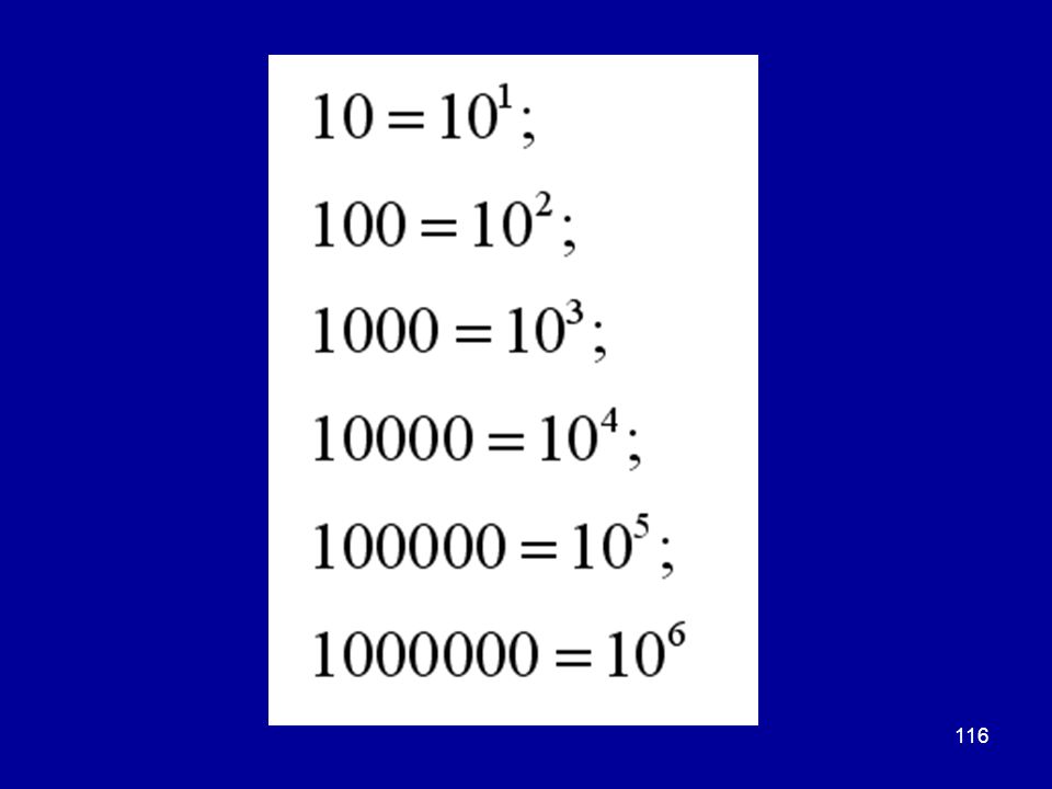
115. A logarithmic system
In a LOGARITHMIC SYSTEM, numbers are expressed as POWERS of a constant known as the BASE.
The numbers 10, 100, 1000, 10,000,
100, 000 and 1, 000,000 can all be expressed as powers of 10 thus:

117. Definition of a log
The log of a number is the power to which the base must be raised to equal the number.
So, since 1000 = 103, the log of 1000 to the base 10 is 3.
The two most common bases are 10 and the number e, where e ≈ 2.72
Logs to the base e are known as NATURAL LOGS.

119. Notation for logs

120. The antilog

121. The exponential function

122. The laws of logs
The definition of the antilog is the key to the derivation of the LAWS OF LOGARITHMS.
For example, the log of the PRODUCT is the SUM of the logs.

123. Three laws of logs The log of the PRODUCT is the SUM of the logs.
The log of the QUOTIENT is the DIFFERENCE between the logs.
The log of the POWER is the power TIMES the log.

124. Things to remember about logs
There is no log for a negative number.
The log of zero is –∞ (minus infinity).
A log can have a negative value. It does so when the number is a PROPER FRACTION (numerator less than the denominator, so with a value between zero and 1).
The log of 1 is zero.