Bayesian Clinical Trials

Bayesian Clinical Trials
Scott M. Berry 1

Bayesian Statistics Reverend Thomas Bayes (1702-1761)
Essay towards solving a problem in the doctrine of chances (1764) This paper, on inverse probability, led to Bayes theorem, which led to Bayesian Statistics

Bayes Theorem Bayesian inferences follow from Bayes theorem:
'(q| X)  (q)*f (X | q) Assess prior ; subjective, include available evidence Construct model f for data Find posterior ' Both of these tasks are difficult.

Simple Example Coin, P(HEADS) = p p = 0.25 or p =0.75, equally likely.
DATA: Flip coin twice, both heads. p ???

Bayes Theorem Posterior Probabilities Pr[ p = 0.75 | DATA] =
Pr[DATA | p=0.75] Pr[p=0.75] Pr[DATA | p=0.75] Pr[p=0.75] + Pr[DATA | p=0.25] Pr[p=0.25] (0.75)2 (0.5) = 0.90 (0.75)2 (0.5) + (0.25)2 (0.5) Posterior Probabilities Likelihood Prior Probabilities

Rare Disease Example Suppose 1 in 1000 people have a rare disease, X, for which there is a diagnostic test which is 99% effective. A random subject takes the test, which says “POSITIVE.” What is the probability they have X? (0.99) (0.001) = !!! (0.99) (0.001) + (0.01) (0.999)

Bayesian Statistics A subjective probability axiomatic approach was developed with Bayes theorem as the “mathematical crank”--Savage, Lindley (1950’s) Very different than classical statistics: a collection of tools Before ?: A philosophical niche, calculation very hard. Early 1990’s: Computers and methods made calculation possible…and more!

Bayesian Approach Probabilities of unknowns: hypotheses, parameters, future data Hypothesis test: Probability of no treatment effect given data Interval estimation: Probability that parameter is in the interval Synthesis of evidence Tailored to decision making: Evaluate decisions (or designs), weigh outcomes by predictive probabilities

Frequentist vs. Bayesian— Seven comparisons
1. Evidence used? 2. Probability, of what? 3. Condition on results? 4. Dependence on design? 5. Flexibility? 6. Predictive probability? 7. Decision making?

Consequence of Bayes rule: The Likelihood Principle
The likelihood function LX() = f( X | ) contains all the information in an experiment relevant for inferences about  It is important to distinguish between “observed data” and data generally.

Short version of LP: Take data at face value
But “data” can be deceptive Caveats . . . How identified? Why are they showing me this?

Example Data: 13 A's and 4 B's Parameter =  = P(A wins)
Likelihood   13 (1–)4 Frequentist conclusion? Depends on design

Frequentist hypothesis testing
P-value = Probability of observing data as or more extreme than results, assuming H0. P-V = P(tail of dist. | H0) Four designs: (1) Observe 17 results (2) Stop trial once both 4 A's and 4 B's (3) Interim analysis at 17, stop if or A's, else continue to n = 44 (4) Stop when "enough information"

Design (1): 17 results Binomial distribution with n = 17,  = 0.5;
P-value = 0.049

Design (2): Stop when both 4 A’s and 4 B’s
Two-sided negative binomial with r = 4,  = 0.5; P-value = 0.021

Design (3): Interim analysis at n=17, possible total is 44
Analyses at n = 17 & 44; 17 if 0-4 or 13-17; P = 0.085 Both shaded regions = 0.049 P(both) = 0.013; net = 2(0.049) – 0.013 = 0.085

Design (4): Scientist’s stopping rule: Stop when you know the answer
Cannot calculate P-value Strictly speaking, frequentist inferences are impossible

Bayesian Calculations
Data: 13 A's and 4 B's Parameter =  = P(A wins) For ANY design with these results, the likelihood function is P(data | p)   13 (1–)4 Posterior probabilities & Bayesian conclusion same for any design

Likelihood function of 

Posterior Distribution
Prior: <  < 1 Posterior  1 *  13 (1–)4 = 1 *  13 (1–)4 / ∫ 1 *  13 (1–)4 d  = {13!4!/18!}  13 (1–)4

Posterior density of  for uniform prior: Beta(14,5)

Pr[ > 0.5 ]

PREDICTIVE PROBABILITIES
Distribution of future data? P(next is an A) = ? Critical component of experimental design In monitoring trials

Laplace’s rule of succession
P(A wins next pair | data) = EP(A wins next pair | data, ) = E( | data) = mean of Beta(14, 5) = 14/19 Laplace uses Beta(1,1) prior

Updating w/next observation

Suppose 17 more observations
P(A wins x of 17 | data) = EP(A wins x | data, ) =  Beta-Binomial Distribution

Predictive distribution
Predictive distribution of # of successes in next 17 tries: 88% probability of statistical significance Has more variability than any binomial 

Best fitting binomial vs. predictive probabilities
Binomial, p=14/19 96% probability of statistical significance Predictive, p ~ beta(14,5) 88% probability of statistical significance

Possible Calculation Simulate a  from the beta(14,5)
Simulate an x from binomial(17, ) Distribution of x’s is beta-binomial--the predictive distribution

Posterior and Predictive…same?
Clinical Trial, 100 subjects. HA:  > 0.25? FDA will approve if # success ≥ 33 [post > 0.95, beta(1,1)] See 99 subjects, 32 successes Pr[  > 0.25 | data ] = 0.955 Predictive prob trial success = 0.327

Predictive Probabilities for Medical Device
Bayesian calculations  FDA: Some patients have reached 2 years Some patients have only 1-yr follow-up

Continuous data; Patients w/both 12 and 24 months

Some patients with only 12-month data

Kernel density estimates

Small bandwidth (0.2)

Larger bandwidth (0.3)

Still larger bandwidth (0.4)

Very large bandwidth (0.5) (nearly bivariate normal)

Condition on 12-month value

Conditional distribution of 24-month value (0.2)

For largest bandwidth (0.5)

Multiple imputation: simulate full set of 24-month data

Simulate experimental patients and controls in this way— multiple imputation
Make inferences with full data (for example, equivalent improvement) Repeat simulations (≥10,000 times) Gives probability of future results– for example, of “equivalence”

Monitoring example: Baxter’s DCLHb
Diaspirin Cross-Linked Hemoglobin Blood substitute; emergency trauma Randomized controlled trial (1996+) Treatment: DCLHb Control: saline N = 850 (= 425x2) Endpoint: death

Waiver of informed consent
Data Monitoring Committee First DMC meeting: DCLHb Saline Dead 21 (43%) 8 (20%) Alive Total No formal interim analysis

Bayesian predictive probability of future results (no stopping)
Probability of significant survival benefit for DCLHb after 850 patients: (PP=0.0097) DMC paused trial: Covariates? DMC stopped the trial

Herceptin in Neoadjuvant BC
Endpoint: tumor response Balanced randomized, A & B Sample size planned: 164 Interim results after n = 34: Control: 4/16 = 25% (pCR) Herceptin: 12/18 = 67% (pCR) Not unexpected (prior?) Predictive prob of stat sig: 95% DMC stopped the trial ASCO and JCO—reactions …

Mixtures: Data: 13 A's and 4 B's Likelihood  p13 (1–p)4

Mixture Prior p ~ p0 I[p=p0] + (1-p0) Beta(a,b)
p  p0 I0 p013(1-p0)4 + (1-p0) Kpa+13-1(1-p)b+4-1 p ~ p0 I0 + (1-p0) Beta(a+13,b+4 ) p0 p13(1-p)4 p0 = G(a)G(b)G(a+b+17) p0 p13(1-p)4 + (1-p0) G(a+13)G(b+4)G(a+b)

Mixture Posterior p0=.5 Pr(p=0.5) = 0.246 P(p > 0.5) = 0.742

Crooked-Penny Example
Flip the coin 20 times. What is q for your coin? Everyone reports p for their coin. ^ A new estimate for q? Are others relevant for you?

Numbers of heads This is you

One-Sample Problem [q] ~ Beta(a,b) [X] ~ Binomial(n,q)
[q|X]~Beta(a+X,b+n-X) Mean = (a + X)/(a+b+n)

For uniform prior (a = b = 1)
Posterior: q ~ Beta(17, 5) Prior: q ~ Beta(1, 1) 0.77

For a = b = 10 Posterior: q ~ Beta(26, 14) Prior: q ~ Prior: q ~
0.65

Remember the other coins . . .
This is you

Learning about the prior
In your setting the other coins give you information about the prior…which helps!!!! The coins do not have to be the same or close, you learn the appropriate amount of borrowing.

HIERARCHICAL MODELING
Population: Sample: Inferential problems Sample from sample:

Selecting coins Population of coins—population of q’s:
Select two coins and toss each coin 10 times: one 9 heads, other 4 heads. Estimate q1, q2. Estimate distribution of q’s in population.

Generic example: Unit is lab or drug variation or lot or study
Unit s n s/n Total n = #observations s = #successes s/n = success proportion

If q1 = q2 = . . . = q9 = q (all 150 units exchangeable)

Assuming equal q’s, 95% CI for q: (0.63, 0.77)
But 7 of 9 estimates lie outside this interval. Combined analysis unsatisfactory. Nine different analyses even worse: nine individual CIs?

Suppose ni independent observations on unit i
Suppose each unit has its own q, with q1, , q9 having distribution G. Observe x's, not q's. Xi ~ binomial(ni, qi). Likelihood is product of likelihoods of qi

Bayesian view: G unknown = G has probability distribution
Prior distribution reflects heterogeneity vs homogeneity. Assume G is Beta(a,b), a > 0, b > 0 with a and b unknown. Study heterogeneity: little if a+b is large lots if a+b is small

Beta(a,b) for a, b = 1, 2, 3, 4:

Suppose uniform prior for a & b on integers 1, . . ., 10

Posterior probabilities for a & b

Calculating posterior distribution of G
Direct in this example Can be more complicated, and require: Gibbs sampling (BUGS) Other Markov chain Monte Carlo

Posterior mean of G (also predictive density for q)

Contrast with likelihood assuming all p’s equal

Bayesian questions: P(q > 1/2) = ????
P(next unit in study i is success) = ? How to weigh results in unit i? How to weigh results in unit j? P(unit in 10th study is success) = ? How to weigh results in study i?

Bayes estimates Unit x n x/n Bayes 1 20 20 1.00 0.90 2 4 10 0.40 0.53
Total (0.71)

Bayes estimates are regressed or shrunk toward overall mean
Unadjusted estimates

Baseball Example 446 players in 2000 with > 100 at bats Jose Vidro

X ~ Binomial(606, qJV) (hits) qJV ~ Beta(a,b) How good was Jose Vidro?
(200 hits in 606 at bats, 0.330) X ~ Binomial(606, qJV) (hits) qJV ~ Beta(a,b)

Empirical Bayes: aEB = bEB=258.9 (mean = 0.269; var = ) [q|X] ~ Beta( , ) (approx) Posterior mean = 0.308 Posterior st. dev. = 0.015

Science, Feb 6, 2004, pp 784-6

Efficacy of Pravastatin + Aspirin: Meta-Analyses
ohrms/dockets/ac/02/slides/ 3829s2_03_Bristol-Meyers-meta-analysis.ppt Efficacy of Pravastatin + Aspirin: Meta-Analyses [For statistical analysis, S.M. Berry et al., Journal of the American Statistical Association, 2004]

Meta-Analysis of these Pravastatin Secondary Prevention Trials
Number of Subjects* % on Aspirin Primary Endpoint LIPID 9014 82.7 CHD mortality CARE 4159 83.7 CHD death & non-fatal MI REGRESS 885 54.4 Atherosclerotic progression (& events) PLAC I 408 67.5 Atherosclerotic progression (& events) PLAC II 151 42.7 Atherosclerotic progression (& events) Totals 14,617 80.4 *99.7% of pravastatin-treated subjects received 40mg dose

Trial Commonalities Similar entry criteria
Patient populations with clinically evident CHD Same dose of pravastatin (40mg) Randomized comparison against placebo All trials with durations of  2 years Pre-specified endpoints Covariates recorded Common meta-analysis data management

Patient Group Comparisons
Randomized Groups Pravastatin Placebo Aspirin Users Prava+ASA Prava alone Placebo+ASA Placebo alone Randomized Comparison Aspirin Non-Users Observational Comparison

Is Pravastatin+Aspirin More Effective than Pravastatin Alone?
Aspirin studies were conducted before statins were widely used Placebo-controlled trial with aspirin is not feasible Investigation of pravastatin database to explore this question

Is the Combination More Effective than Pravastatin Alone?
Unadjusted event rates in LIPID and CARE suggest pravastatin + aspirin is more effective than pravastatin alone

Event Rates for Primary Endpoints in LIPID and CARE
Pravastatin-treated Subjects Only Trial: Primary Endpoint: LIPID CHD Death CARE CHD Death or Non-fatal MI Aspirin Users 5.8% 8.8% Observational Comparison 14.8% 9.3% Aspirin Non-Users

Accounting for Baseline Risk Factors
Age Gender Previous MI Smoking status Baseline LDL-C, HDL-C, TG Baseline DBP & SBP Additional analyses also included revascularization, diabetes and obesity

Meta-Analysis Endpoints Considered
Fatal or non-fatal MI Ischemic stroke Composite: CHD death, non-fatal MI, CABG, PTCA or ischemic stroke

H(t) = l0(t)exp(Zb + fS + gT)
Meta-Analysis Models Model 1: Multivariate Cox proportional hazards model Patients combined across trials; trial effect is a fixed covariate H(t) = l0(t)exp(Zb + fS + gT) Covariates Baseline Hazards constant Study effects Treatment Effects

Relative Risk Reduction Cox Proportional Hazards – All Trials
Prava+ASA vs ASA alone Prava+ASA vs Prava alone Fatal or Non-Fatal MI 0.400 0.800 1.000 0.600 Relative Risk (95% CI) RRR 31% 0.69 26% 0.74 Prava+ASA vs ASA alone Prava+ASA vs Prava alone 29% 0.71 31% 0.69 Ischemic Stroke 0.400 0.800 1.000 0.600 0.400 0.800 1.000 0.600 CHD Death, Non-Fatal MI, CABG, PTCA, or Ischemic Stroke Prava+ASA vs ASA alone Prava+ASA vs Prava alone 24% 0.76 13% 0.87 RRR = Relative Risk Reduction

H(t) = l0(t)exp(Zb + fS + gT)
Meta-Analysis Models Model 2: Same as Model 1 except Allows trial heterogeneity: Bayesian hierarchical (random effects) model of trial effect H(t) = l0(t)exp(Zb + fS + gT) Covariates Baseline Hazards piecewise-constant Study effects Hierarchical Treatment Effects

Model 2 – Hierarchical, Random Effects
Fatal or Non-Fatal MI 0.000 0.025 0.050 0.075 0.100 1 2 3 4 5 Placebo Prava alone ASA alone Prava+ASA Cumulative Proportion of Events Year

Ischemic Stroke Only 0.000 0.005 0.010 0.015 0.020 0.025 1 2 3 4 5 Prava alone Placebo ASA alone Prava+ASA Cumulative Proportion of Events Year

CHD Death, Non-Fatal MI, CABG, PTCA, or Ischemic Stroke 0.00 0.05 0.10 0.15 0.20 0.25 1 2 3 4 5 Year Prava alone Placebo Prava+ASA ASA alone Cumulative Proportion of Events

Combination is More Effective than Either Agent Alone
Pravastatin + aspirin provides benefit for all three endpoints: 24% - 34% RRR compared with aspirin 13% - 31% RRR compared with pravastatin This benefit was similar in Models 1 and 2 This benefit was consistent in both LIPID and CARE trials

Model 2: Fatal or Non-Fatal MI
Cumulative Proportion of Events 0.000 0.025 0.050 0.075 0.100 Year 1 2 3 4 5 Prava+ASA ASA alone Prava alone Placebo 0.000 0.005 0.010 0.015 0.025 Year 1 2 3 4 5 0.020 Hazard Prava+ASA ASA alone Prava alone Placebo

H(t) = lT0(t)exp(Zb + fS)
Meta-Analysis Models Model 3: Same as Model 2 except Treatment hazard ratios vary over time H(t) = lT0(t)exp(Zb + fS) Baseline Hazards piecewise-constant Within treatment Covariates Study Effects Hierarchical

Model 3: Fatal or Non-Fatal MI
Cumulative Proportion of Events 0.000 0.025 0.050 0.075 0.100 Year 1 2 3 4 5 Prava+ASA ASA alone Prava alone Placebo 0.000 0.005 0.010 0.015 0.030 Year 5 Separate Analyses: One per Year 1 2 3 4 5 0.020 Hazard 0.025 Prava+ASA ASA alone Prava alone Placebo

Probability of synergy between pravastatin & aspirin
Endpoint Model 2 Model 3 All events 0.983 0.985 Cardiac events 0.945 0.947 Any MI 0.911 0.923 Stroke 0.924 0.906 Death 0.997

Conclusion of Hazard Analysis over Time
Benefit of pravastatin+aspirin over aspirin was present in each year of the 5-year duration of the trials Benefit of pravastatin+aspirin over pravastatin was present in each year of the 5-year duration of the trials Benefits estimated from Model 1 (and confidence intervals) confirmed by more general models and fewer assumptions

Hierarchical modeling in design
Using historical information Combining results from multiple concurrent trials (or many centers)

Hierarchical modeling & dose-response
Example: drug Z (rozuvastatin) vs drug A (atorvastatin) (Berry et al., 2002, American Heart Journal)

Studies involving drugs A and Z*, with %change from baseline.
Study n Dose Mean SD Y – 45 20 – – Placebo – – 16 20 – 12 80 – – – – – Placebo – Placebo 18 10 – – – 51 20 – 61 40 – 10 80 –

Study n Dose Mean SD Y – –37.6 NA 0.624 Placebo – – 11 10 – 10 20 – 11 40 – 11 80 – – –46 NA 0.54 Placebo 15 10 – 13 80 – 14 1* – * – 16 5* – 17 10* – 17 20* – 18 40* – Placebo 15 40* – 31 80* –

Dose-response model Yij = exp{as + at + bt log(d)} + eij s for study
t for drug d for dose i for observation (1, , 43) j for patient within study/dose eij is N(0, s2) Priors don’t matter much, except . . .

Prior for as ~ N(0, t2) t2 is important
t2 large means studies heterogeneous—little borrowing t2 small means studies homogeneous—much borrowing Prior of t2 is IG(10, 10) Prior mean and sd are 0.10 & 0.017

Likelihood Calculations of posterior & predictive distributions by MCMC

Posterior means and SDs
Parameter Mean StDev aP – aA – aZ – bA – bZ – s t

Posterior means and SDs
Par. Mean StDev Par. Mean StDev a a10 – a2 – a a a12 – a4 – a13 – a5 – a a6 – a a a16 – a a17 – a9 –

Model fit

Interval estimates for pop. mean: model (line) vs standard (box)

Study/dose-specific interval estimates: model (line) vs standard (box)

Posterior dist’n of reduction (95% intervals)
Drug A Drug Z

Posterior dist’n of mean diff, A – Z

Really neat . . . Using predictive probabilities for designing future studies Contour plots

Observed %Y for future study with nA=nZ=20 dA=dZ=10

Observed %Y for future study with nA=nZ=100 dA=dZ=10

Observed %Y for future study with nA=nZ=20 dA=10, dZ=5

Observed %Y for future study with nA=nZ=100 dA=10, dZ=5

STELLAR trial results (each n≈160)
Predicted atorva -36% Predicted rosuva -41% -46% -50% -52% -54% -58%

Posterior dist’n of reduction (95% intervals)
Recall: Drug A Drug Z

Adaptive Phase II: Finding the “Best” Dose
Scott M. Berry

Standard Parallel Group Design
Equal sample sizes at each of k doses. Doses 7

True dose-response curve (unknown)
Doses 7

Observe responses (with error) at chosen doses
7

Dose at which 95% max effect
Response True ED95 Doses 8

Uncertainty about ED95 Response ? Doses 7

Increase number of doses
Solution: Increase number of doses Response True ED95 Doses 8

But, enormous sample size, and . . . wasted dose assignments—always!
Response True ED95 Doses 8

Solutions Lots of doses (continuum?) Adaptive Allocation
Model dose response Define what you are looking for Stop when you find what you are looking for… Yogi Berra-ism: If you don’t know where you are going, how do you know when you get there?

Dose Finding Trial Real example (all details hidden, but flavor is the same) “Delayed” Dichotomous Response (random waiting time) Combine multiple efficacy + safety in the dose finding decision Use utility approach for combining various goals Multiple statistical goals Adaptive stopping rules

Adaptive Approach

Statistical Model The statistical model captures all the uncertainty in the process. Capture data, quantities of interest, and forecast future data Be “flexible,” (non-monotone?) but capture prior information on model behavior. Invisible in the process

Empirical Data Observe Yij for subject i, outcome j
Yij = 1 if event, 0 otherwise j = 1 is type #1 efficacy response j = 2 is type #2 efficacy response j = 3 is minor safety event j = 4 is major safety event

Efficacy Endpoints j(d) ~ N(j, 2) Let d be the dose
Pj(d) probability of event j, dose d. j(d) ~ N(j, 2) G(1,1) N(1,1) N(–2,1) IG(2,2)

Safety Endpoint Let di be the dose for subject i
Pj(d) probability of safety j, dose d. N(-2,1) G(1,1) N(1,1)

Utility Function Multiple Factors: Utility is critical: Defines ED?
Monetary Profile (value on market) FDA Success Safety Factors Utility is critical: Defines ED?

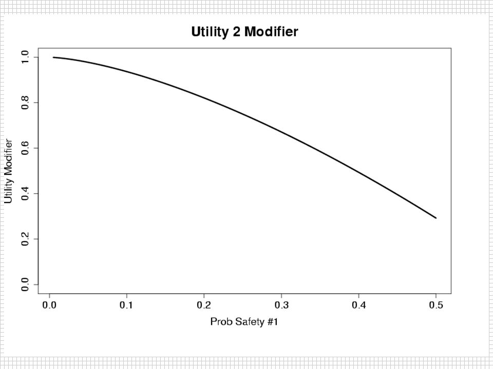
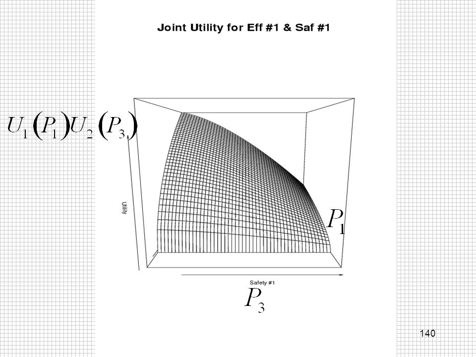
U(d)=U1(P1)U2(P3)*U3(P0,P2)*U4(P4)
Utility Function U(d)=U1(P1)U2(P3)*U3(P0,P2)*U4(P4) Monetary FDA Approval Extra Safety P0 is prob efficacy 2 success for d=0

Monetary Utility

U3: FDA Success “DSMB?”

Statistical + Utility Output
E[U(d)] E[j(d)], V[j(d)] E[Pj(d)], V[Pj(d)] Pr[dj max U] Pr[P2(d) > P0] Pr[ P2 >> P0 | 250/per arm) each d >> means statistical significance will be achieved

Allocator Goals of Phase II study? Find best dose?
Learn about best dose? Learn about whole curve? Learn the minimum effective dose? Allocator and decisions need to reflect this (if not through the utility function) Calculation can be an important issue!

Allocator d* is the max utility dose, d** second best Find best dose?
Learn about best dose? d* is the max utility dose, d** second best Find the V* for each dose ==> allocation probs

Allocator V*(d≠0) = V*(d=0) =

Allocator “Drop” any rd<0.05 Renormalize

Decisions Shut down allocator wj if stop!!!!
Find best dose? Learn about best dose? Shut down allocator wj if stop!!!! Stop trial when both wj = 0 If Pr(P2(d*) >> P0) < 0.10 stop for futility If found, stop: Pr(d = d*) > C1 If found, stop: Pr(P2(d*) >> P0)>C2

More Decisions? Ultimate: EU(dosing) > EU(stopping)?
Wait until significance? Goal of this study? Roll in to phase III: set up to do this Utility and why? are critical and should be done--easy to ignore and say it is too hard.

Simulations Subject level simulation
Simulate 2/day first 70 days, then 4/day Delayed observation exponential with mean 10 days Allocate + Decision every week First 140 subjects 20/arm

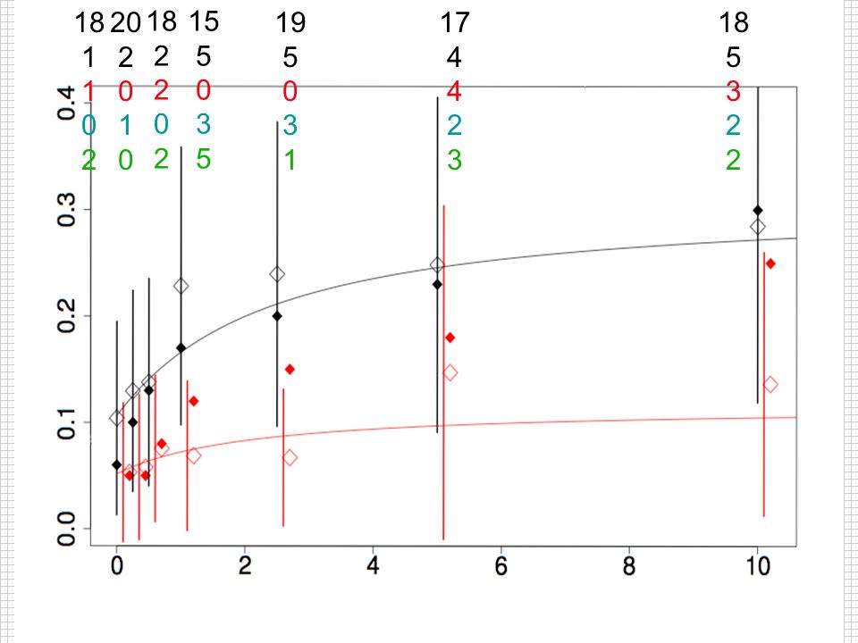
Scenario #1 Stopping Rules: C1 = 0.80, C2 = 0.90 Dose P1 P2 P3 P4 UTIL
0.06 0.05 0.25 0.10 0.5 0.13 0.08 0.07 0.063 1 0.17 0.12 0.323 2.5 0.20 0.15 0.09 0.457 5 0.23 0.18 0.532 10 0.30 0.11 0.656 MAX Stopping Rules: C1 = 0.80, C2 = 0.90

18 1 2 20 2 1 18 2 15 5 3 19 5 3 1 17 4 2 3 18 5 3 2

Dose Probabilities .25 .5 1 2.5 5 10 .18 .33 .27 .29 .67 P(max) .01
.25 .5 1 2.5 5 10 P(>>Pbo) .18 .33 .27 .29 .67 P(max) .01 .04 .06 .52 P(2nd) .03 .10 .13 .35 .32 Alloc .02 .46

20 1 3 20 2 1 18 2 19 5 1 4 19 5 3 25 7 8 2 24 7 5 2

.25 .5 1 2.5 5 10 P(>>Pbo) .12 .38 .36 .92 .91 P(max) .00 .02 .04 .41 .53 P(2nd) .03 .06 .07 .47 .37 Alloc .09 .34 .51

21 2 1 20 2 1 19 3 2 1 20 5 1 4 21 5 3 4 29 7 9 2 11 31 11 6 3 17

Dose Probabilities .25 .5 1 2.5 5 10 .13 .39 .38 .26 .97 .85 P(max)
.25 .5 1 2.5 5 10 P(>>Pbo) .13 .39 .38 .26 .97 .85 P(max) .00 .02 .03 .01 .55 P(2nd) .10 .05 .46 .35 Alloc .11

23 2 1 4 20 2 1 20 4 2 21 5 1 4 25 5 1 4 36 7 10 3 45 12 10 3 16

.25 .5 1 2.5 5 10 P(>>Pbo) .16 .41 .38 .48 .93 P(max) .00 .02 .03 .04 .26 .65 P(2nd) .05 .07 .10 .49 .29 Alloc .08 .11 .18 .35 .28

26 2 1 20 2 1 20 4 2 25 5 1 4 6 26 6 2 4 5 44 7 13 3 12 52 13 10 4 15

Dose Probabilities .25 .5 1 2.5 5 10 .16 .40 .31 .41 .98 .89 P(max)
.25 .5 1 2.5 5 10 P(>>Pbo) .16 .40 .31 .41 .98 .89 P(max) .00 .02 .03 .06 .27 .63 P(2nd) .12 .48 .28 Alloc .10 .04 .13 .26 .30

26 2 1 6 20 2 1 21 4 2 3 26 6 1 4 5 33 7 3 4 5 52 8 13 4 10 61 18 15 4 12

.25 .5 1 2.5 5 10 P(>>Pbo) .13 .36 .32 .65 .96 P(max) .00 .01 .09 .08 .81 P(2nd) .05 .23 .52 .15 Alloc

Trial Ends P(10-Dose max Util dose) = 0.907
P(10-Dose >> Pbo 250/arm) = 0.949 280 subjects: 32, 20, 24, 31, 38, 62, 73 per arm

Operating Characteristics
Pbo 0.25 0.5 1 2.5 5 10 SS 39 21 25 37 63 89 110 Pmax --- 0.00 0.04 0.96 66 0.01 0.06 0.93

Adaptive Constant P(Success) 0.936 0.810 P(Cap) 0.064 0.190 P(Futility) 0.000 Mean SS 384 459 SD SS 186 224 Mean TDose 1754 1263 Max TDose 4818 2370

0.06 0.05 0.25 0.10 0.5 0.13 0.08 0.07 0.063 1 0.17 0.12 0.323 2.5 0.20 0.15 0.452 5 0.23 0.18 0.502 10 0.40 0.302 Stopping Rules: C1 = 0.80, C2 = 0.90

Pbo 0.25 0.5 1 2.5 5 10 SS 71 27 41 81 137 172 164 Pmax --- 0.00 0.03 0.22 0.60 0.16 100 0.20 0.44 0.33

Adaptive Constant P(Success) 0.314 0.266 P(Cap) 0.686 0.734 P(Futility) 0.000 Mean SS 694 702 SD SS 193 190 Mean TDose 2954 1937 Max TDose 4489

Simulation #3 Stopping Rules: C1 = 0.80, C2 = 0.90 Dose P1 P2 P3 P4
UTIL 0.06 0.05 0.1 0.10 0.5 0.13 0.08 0.07 0.063 1 0.30 0.25 0.11 0.656 2.5 0.17 0.12 0.323 5 0.20 0.15 0.09 0.457 10 0.23 0.18 0.532 Stopping Rules: C1 = 0.80, C2 = 0.90

Pbo 0.25 0.5 1 2.5 5 10 SS 53 23 28 119 52 76 102 Pmax --- 0.00 0.92 0.01 0.07 87 0.83 0.02 0.15

Adaptive Constant P(Success) 0.906 0.596 P(Cap) 0.092 0.404 P(Futility) 0.002 0.000 Mean SS 453 606 SD SS 187 205 Mean TDose 1663 1662 Max TDose 3771

0.06 0.05 0.25 0.5 1 2.5 0.20 0.10 0.573 5 10 Stopping Rules: C1 = 0.80, C2 = 0.90

Pbo 0.25 0.5 1 2.5 5 10 SS 53 21 22 23 150 160 163 Pmax --- 0.00 0.27 0.32 0.40 92 0.28 0.33

Adaptive Constant P(Success) 0.514 0.408 P(Cap) 0.486 0.592 P(Futility) 0.000 Mean SS 591 647 SD SS 239 220 Mean TDose 2840 1780 Max TDose 4815

0.06 0.05 0.1 0.07 0.5 0.08 1 0.09 2.5 5 0.10 10 0.11 Stopping Rules: C1 = 0.80, C2 = 0.90

Pbo 0.25 0.5 1 2.5 5 10 SS 92 91 75 66 76 83 90 Pmax --- 0.45 0.04 0.07 0.10 0.13 0.21 84 0.44 0.08 0.12 0.15 0.17

Adaptive Constant P(Success) 0.004 0.006 P(Cap) 0.484 0.544 P(Futility) 0.512 0.450 Mean SS 574 589 SD SS 250 258 Mean TDose 1637 1615 Max TDose 3223.5

0.06 0.05 0.1 0.5 1 2.5 5 Stopping Rules: C1 = 0.80, C2 = 0.90

Pbo 0.25 0.5 1 2.5 5 10 SS 66 77 51 34 38 41 43 Pmax --- 0.90 0.01 0.02 0.03 56 0.86 0.05

Adaptive Constant P(Success) 0.000 P(Cap) 0.122 0.190 P(Futility) 0.878 0.810 Mean SS 350 395 SD SS 215 241 Mean TDose 811 1086 Max TDose 2404

Bells & Whistles Interest in Quantiles Minimum Effective Dose
“Significance,” control type I error Seamless phase II --> III Partial Interim Information “Biomarkers” of endpoint Continuous (& Poisson) Continuum of doses (IV)--little additional n!!!

Conclusions Approach, not answers or details!
Shorter, smaller, stronger! Better for company, FDA, Science, PATIENTS Why study?--adaptive can help multiple needs. Adaptive Stopping Bid Step!

Bayesian Clinical Trials

Similar presentations

Presentation on theme: "Bayesian Clinical Trials"— Presentation transcript:

Similar presentations

About project

Feedback

Log in

Auth with social network:

Bayesian Clinical Trials

Similar presentations

Presentation on theme: "Bayesian Clinical Trials"— Presentation transcript:

Similar presentations

About project

Feedback