1. Noises : From Physics to Biology
卓 益 忠
北方温泉会议中心

2. 隔行如隔山 Crossover Sciences
Mountain in Between
隔行如隔山
To climb over or penetrate through the mountain between physics and biology, the noises play a crucial role: noise assisting tunneling and climbing.

3. Part 1,Noise in Physics 1, Phenomenological Theories
(A),布朗运动(Brownian Motion)
(B) 牛顿与朗之万之间（Intermediate Dynamics between Newton and Langevin)
2, 微观动力学基础(Microscopic Foundation)

4. Part 2, Noise in Biology
1, Complex dynamics of life at different scales
(A), Biological response to radiation
(B),主动布朗运动(Active Brownian motion)
2, New approaches to the solutions of noisy biological networks
3, Fluctuation-Dissipation Theorem
4, Signal Transduction
5, Perspective

5. (A)布朗运动(Brownian Motion)
Part 1,Noise in Physics
1,Phenomenological Theories
(A)布朗运动(Brownian Motion)
最简单的一种随机行走(random walks)
自然界中(物理,化学与生物等)普遍存在
广泛应用于原子核大振幅运动(核裂变, 核融合)的输运理论 及各种生物过程。

6. Brownian Motion phenomenon was discovered by the Scottish botanist Robert Brown in 1827.
The first quantitative explanation of Brownian motion was due to Einstein in 1905.
In his picture the spatial position of a Brownian particle was a stochastic process.

7. The beauty of Einstein’s model is that it permits a quantitative comparison to experiment.
Einstein’s quantitative explanation for Brownian motion put the long standing discussion on the molecular nature of matter to rest, thus to start a new era for the science of life.
At the same time, he set the cornerstone for the development of statistical mechanics.

8. Delbrueck et al suggested the molecular nature of genetic code in 1935.
Schrodinger deduced that the gene was an aperiodic crystal composed of a linear array of different isomeric component in his book What is life(1944)
The structure of DNA was solved by Watson and Crick in 1953, and thus a new era of molecular biology started.

9. The diffusion constant for spheres of radius R is given by so-called Stockes-Einstein formula:
Einstein’s picture of Brownian motion keeps track only of the position of Brownian particle and ignores the positions and momenta of all the water molecules, as well as the momentum of the particle itself.

10. This, in fact, leads to an unphysical result for the average velocity of the particle, pointed out by Einstein.
A simple way to remedy this situation was taken by Langevin in 1907.Langegevin’s approach was to consider the mechanical equation by separating the force into three parts, in addition to original Newtownian force, there are viscous forces that tend to damp the motion of the particle and the random forces, which are rapid and unpredictable.

11. 2, 微观动力学基础(Microscopic Foundation)

12. Dividing the total system into system plus environment ( reservoir, heat bath) is an universal approach ( open system):
系统＋环境（动力学体系）
应用投影算符（时间无关与时间有关）
（耦合）主方程

13. When the environment is time independent ( heat bath) the time independent projection operator method is used:
Projecting on total density matrix starting from Von Neumann equation
( Schrodinger Representation)
(Nakajima-Zwanzig)
The generalized Master equation is obtained for density matrix of the system.

14. Projecting on the dynamical variable for the total system starting from Heisenberg equation
(Heisenberg Representation)
( H. Mori)
The generalized Langevin Equation is obtained.

15. When environment is time-dependent, the time-dependent projection operator method is to be used both in Schrodinger Representation as well as in Heisenberg Representation.
The coupled Master equations or the coupled Langevin-type equations are obtained.
Due to complication, most derivations are remained in formulations.
We have been interested in this field for a long time.

16. The newest version on this subject by F.Sakata et al:
The main idea is to develop a sort of interaction representation (IR) for a complex system, namely, to treat the irrelevant subsystem by a density matrix, while the relevant subsystem by a dynamical variables.

17. Part 2, Noise in Biology

18. 1, Complex dynamics of life at different scales
(A), Biological response to radiation
(B),主动布朗运动(Active Brownian motion)
2, New approaches to the solutions of noisy biological networks
3, Fluctuation-Dissipation Theorem
4, Signal Transduction
5, Perspective

19. 1, Complex dynamics of life at different scales
It is not within our reach to accurately model the entire living cell, or even an entire process such as the mechanical response or radiation response.
The so called bottom-up approach is now a well-accepted method in all of biophysics. The principal idea is to build models from a limited number of basic components.

20. Once these components are experimentally and theoretically analyzed in detail, the next ingredient is added until celled-like structures are created in a controlled function.
As a result of a bottom up approach, deeper insight into both established mechanisms and new mechanisms may arise.

21. A, Biological response to radiation
Exposure of the cells to ionizing radiation initiates a complex series of physical, chemical, and biological changes that may lead to cell death, organ dysfunction, or cancer.
The responses to such a radiation are at different scales both at time scale and at spatial scale.

22. From radiation induced DNA damage to the observable biological endpoint involves many spatial and temporal scales of different orders of magnitude.

23. Central Dogma DNA RNA Protein Mutation  DNA polymerase: proofreading
Transcription
Translation
DNA
RNA
Protein
Replication
DNA polymerase: proofreading
RNA polymerase: without proofreading
The RNA polymerase is unable to “proofread” during transcription.
This enables the virus to alter surface antigens and accounts for its ability to evade the immune system.
Mutation 

24. DNA is assumed to be the key target as it carries message of life.
Approximations (zero order)
DNA is assumed to be the key target as it carries message of life.
DSB is considered to be the most critical initial damage (neglecting other kind of damage) responsible for subsequent biological effects.

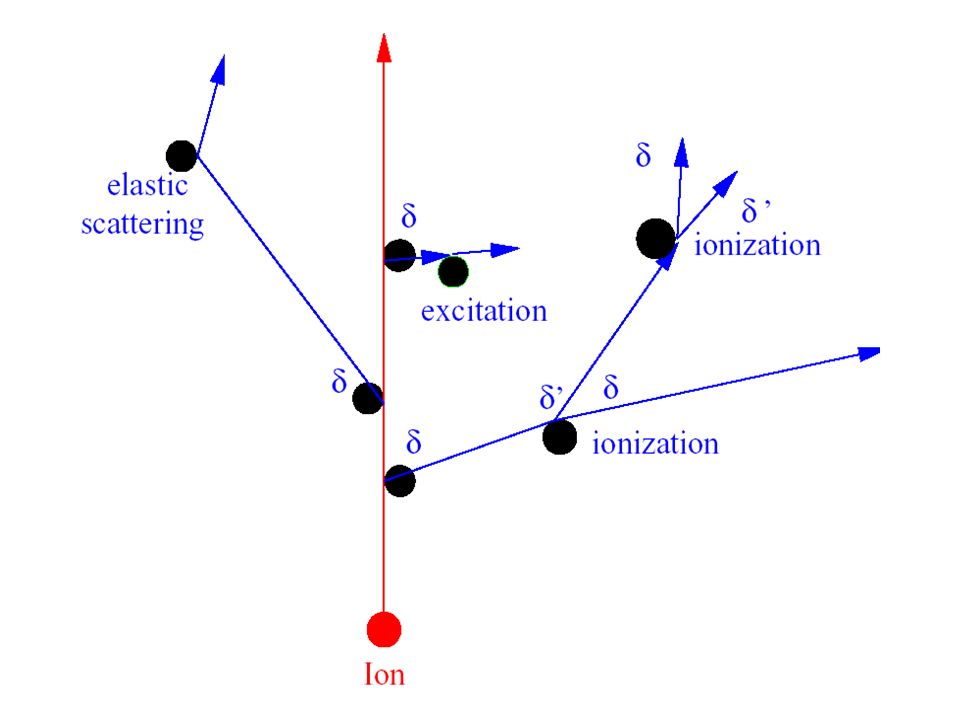
27. Track structure model
Primary energy transfer events (excitation and ionization) occur within 10-10s after radiation passes through a medium(cell).
Deposition of energy is a stochastic (quantum mechanical) process, and its spatial distribution is called track structure.
It is based on the event by event Mote Carlo method to give the spatial distribution of the energy deposit in the nanometer scale and evolution with time in the scale of pico second.

30. Track structure model is one of the most important theoretical tools for studying radiation damage.
Track structure is nano-meter scale dosimetry can provide the spatial distribution of the energy deposit in the scale of nano-meter (dose distribution) which is the basis for studying the DNA damage and also for making plan of cancer radiation therapy

31. . So far, track structure model is still incomplete, within this model medium is mostly treated as water vapor, and the cutoff energy of secondary electron is >10eV
Nuclear process such as fragmentation might be important
More and better cross section data are always needed.

32. From Track Structure to Cell Survival

33. The DNA damage spectra produced by ionizing radiation is often obtained from track structure in water combined with geometrical models of the DNA.
These spectra can be provided as the input data for the phenomenological dynamical models to bridge the physical stage and the biological stage.

34. Biological Network Biochemical networks Example :P53-Mdm2 interaction
Cell is best described as a complex network of chemicals (proteins) connected by chemical reactions.
A network consists of nodes connected by links.

35. The networks have complex topology
The networks have complex topology. Biological networks share common topological features with non-biological networks (Small world, scale free,etc.).

36. Network Motifs
One of the major goals in systems biology is to understand complex protein networks within living cells. Great simplification would occur if networks could be broken down into basic building block, such as recently defined ‘network motifs’.
DNA Damage Network & p53-Mdm2 Interaction-A good example how to treat a complex system in a simple way (network motifs).

37. P53 Tumor Supressor
Input Signal +

38. The Important Functions of P53
The P53 tumor-suppressor gene integrates numerous signals that control cell life and death.
P53 genes act as brakes to the cycle of cell growth, DNA replication and division into two new cells.

39. 激活P53的上游事件 １离子辐射造成的DNA 损伤激活． ATM,Chk2参与 ２化学药物，紫外线，蛋白激酶抑制剂诱导
ATR ,Casein参与
３异常细胞生长
p14ARF参与
三条途径最终都会抑制蛋白的降解，使P53维持高水平，P53通过调节周围基因的表达，行使抑制细胞分裂和促进细胞调亡的功能．

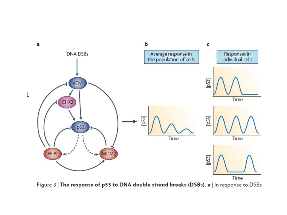
40. P53 dynamics
P53 acts as a node for integrating the incoming damage signal and its primary function is to act as a transcription factor.
The biological end-points of P53 induction are growth arrest or apoptosis.

42. Previous works on the p53-MDM2 interaction that gives damped oscillations in a population of cells
a, Generation of oscillations by the p53-Mdm2 feedback loop :A theoretical and experimental study Ruth Lev Bar-Or et al,PNAS,97(2000)11250

43. Experimental Results by Ruth Lev Bar-Or

44. Theoretical results by Ruth Lev Bar-Or damped oscillation

45. Lahav et al set out to address what was happening in individual cells using fluorescently labeled versions of p53 and Mdm2 that can be visualized and quantified (2004).
They found that, in response to ionizing radiation, p53 was expressed a series of discrete pulses.Genetically identical cells had different numbers of pulses: zero,one,two or more.
The mean height and duration of each pulse were fixed and did not depend on the amount of DNA damage.

46. The mean number of pulses, however, increased with DNA damage.
The suggests that the p53-Mdm2 feedback loop generates a ‘digital’ clock that releases well-timed quanta of p53 until damage is repaired or the cell dies.
Different cells from the same clone in the same field of view showed different numbers of oscillations (Figs. a-c).Figs. d-e shows a cell with two pulses, p53-CFP first appeared in the nucleus, followed, after a delay, by Mdm2-YFP.

47. p53-MDM2 dynamics in single cells under stress
MCF-7 cells,
Lahav et al,
Nat. Genet. 2004

48. The cells tend to show more pulses as damage increases
The cells tend to show more pulses as damage increases. The mean height and width of each pulse was constant and did not depend on irradiation dose.

49. “Analog”
“Digital”

50. p53-Mdm2 负反馈环
suppress
promote
实验观测：
在DNA受到损伤时，p53以一系列脉冲进行表达。每一个峰的高度和宽度大致是固定的，不依赖于DNA的受损程度。但峰的平均数量却依赖于DNA的受损程度。

51. 确定性模型 考虑单个细胞情形： 山形函数 (延迟负反馈) 信号函数
Shiwei Yan, Yizhong Zhuo. Physica D, 2006, 220(2):

52. New Experiments (fluctuation)(2006)
Some cells, damaged by either 5 or 10Gy, show sustained oscillations for the entire time of observation (up to 10 peaks in 60 h). Peak amplitude is highly variable, whereas peak timing is more precise.
Radiation dose determines not the number of pulses but rather the probability that an irradiated cell oscillates permanently or not.

53. Whether the damage is large, small or nonexistent, some cells show “irregular” fluctuations of p53 and Mdm2 with a broad distribution of interpulse intervals from 8–12 h. (Some cells show non-oscillatory fluctuations)

54. 随机性模型 其中

55. The different dynamics of P53 in individual cells in response to UV with a single pulse that increases in amplitude and duration in proportion to the UV dose are observed.
This response contrasts with the previous described series of fixed pulse in response to -radiation.
It is also found that while -triggered P53 pulses are excitable, the P53 response to UV is not excitable and depends on continuous signaling from the input-sensing kinaises.

57. Newest experiment on the response of of P53 to UV radiation (2011)

59. Discussions
a, The behaviors of the oscillations is different for a population of cells (damped)and individual cell (sustained) can be described in a unified way by the proposed dephasing consideration.
This consideration may be too simple! (synchronization and coupling?)
b, Following the “bottom-up approach” P53-Mdm2 feedback loop is only a small part of the DNA damage network , how to take account of the rest part of the network step by step and what is the dynamical behavior of the additional components in the p53 dynamical network.?

60. c, The different dynamical behaviors due to the different kinds of stimulation and different kinds of target cell ,just like the problem of the “combination of the projectiles and targets” in nuclear physics are needed to be further explored both experimentally and theoretically.
d, It is still far away from full understanding of the radiation response at cell level, even at molecular level! A recent report that mutated p53 protein can gain new function and also behave as an oncogene.

61. Molecular Motor (B) 主动布朗运动(Active Brownian motion)
Surprised at the mechanism how the chemical energy is converted into directed motion (mechanical energy) with such high efficiency.
It became a hot topic in last 90s.

62. Dozens of different motor proteins coexist in every eucaryotic cell.
They differ in the type of filament they bind to(either actin or microtubules), the direction they move along the filament, and the “cargo” they carry.
They carry membrane-enclosed organeles-- such as mitochondria , Golgi stacks, or secretory vesicles to their appropriate locations in the cell.

63. All kind of these remarkable motor proteins bind to a polarized cytoskeletal filament and use the energy derived from repeated cycles of ATP hydrolysis to move steadily along it through a large-scale conformational change in a motor protein.
Through a mechanical cycle consisting a few state, the motor protein and its associated cargo move one step at a time along the filament (~ typically a few nanometers).

64. ATP—adenosine triphosphate (三磷酸腺苷)
Figure Molecular Biology of the Cell (© Garland Science 2008)

66. (1), Introduction: Typical example of development along
Tech Exp theories
Last decade :
Optical tweezers, Video microscopy etc.
Single molecular assays: (resol.nm, ms)
Structure (conformational changes),
Kinetics: V~ATP, V~Loads (low),
Energetic: Efficiencies

67. Physical Considerations
Theoretical models:Brownian motors
~Brownian rectifier
Physical Considerations
(1)Small size ~ 100Å (10nm),
(2)Large Brownian Motion,
(3)Binding energy ~ kT,
(4)Nonequilibrium at each Protein site
ATP →ADP +Pi
(5)Filaments are periodic and rigid polar structures
Small machines with large noise

68. Brownian motors consist of three basic ingredients:
asymmetric periodic potential (ratchet potential)
stochastic forces due to thermal fluctuations
various non-equilibrium sources, which lead to various models

69. Most Successful Models:
(Mainly on kinetics)
1, Flashing ratchet model
( More mechanical )
2, Master equation approaches
(More chemical)
They can explain experimental data well!
3, Their relationship is needed to be further explored!

70. (2), Discussions and Perspectives
New challenge and opportunity!
1,To apply the ratcheting mechanism to various problems, such as translocation of proteins across membranes through a nanopore.
2,To describe the behavior of groups of molecular motors, in particular the mechanism of coordination between molecular motors,as molecular motors do not work in isolation but in groups in vivo.

71. In muscles, the number of myosins can reach a few ,even in intracellular transport, about 10 motors coordinate their motion in order to transport vesicles.
“More is different.”
Theoretical models have shown that interaction between motors can lead to nontrivial collective behaviors which cannot be explained by only considering the behavior of an individual motor. These effects include bidirectional motion, oscillations, hysteresis and the formation of dynamical patterns.

72. However, the collective effects due to dynamical phase emerge naturally in the limit of an infinite number of motors for which fluctuations average out.
More precise theories considering a finite number of motors are clearly needed to bridge the gap between single molecule descriptions and the limit of large motor collections.

73. α = 1.5 (superdiffusion)
Phys.Rev.Lett.85,5655(2000)

74. Sub-diffusive motion of RNA molecules in the cell.
Phys.Rev.Lett.96,098102(2006)

77. (3), Collective cell migration
A number of biological processes, such as embryo development, cancer metastasis or wound healing, rely on cells moving in concert. The mechanisms leading to the emergence of coordinated motion remain however largely unexplored.

78. C,Perspective:
Biological problems are full of mysteries.
Despite all of progress has been made so far, the question “What is life” remains.
In a living system we need such a theory :given the conditions of a living system at t1 , one would be able to make a quantitative prediction about that system at t2 , when it runs out of something or other.
Equations of Life!

79. According Feynman’s idea of understanding: “ That which I cannot create I do not understand”.
Learning by building!
We are much better at taking cells apart(top down) than putting them together (bottom up).
Reconstitution of biological processes from component molecules has been a powerful but difficult approach to studying functional organization in biology.

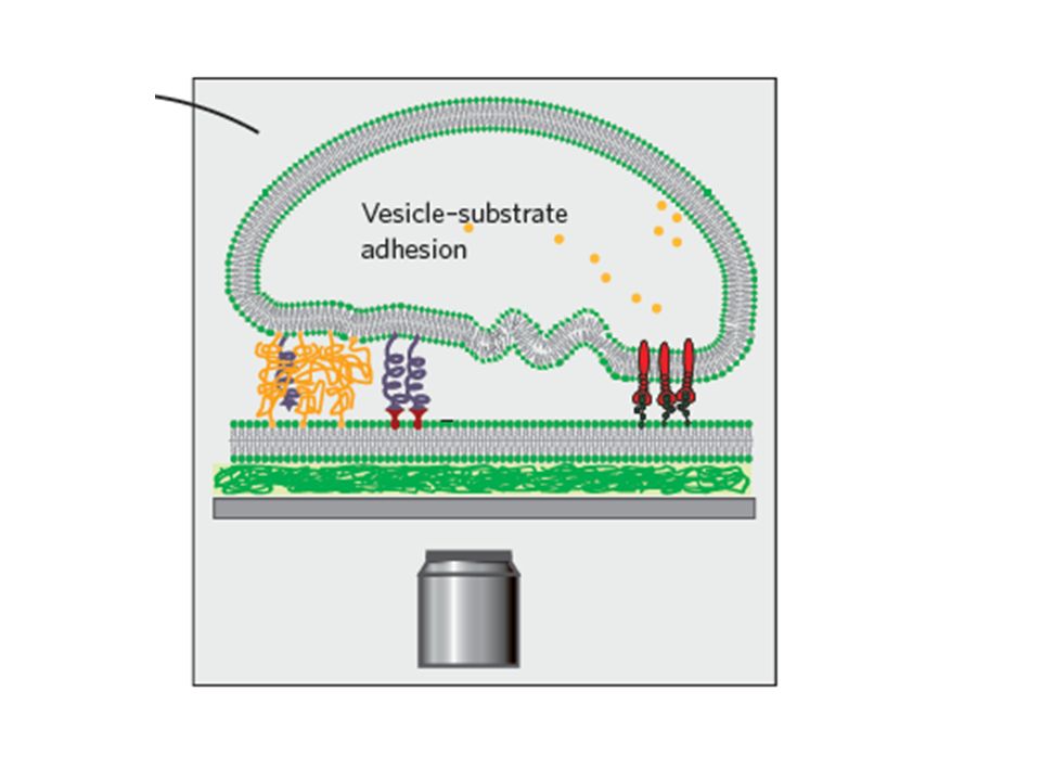
80. The coupling of the membrane (the sensory organ) and the cytoskeleton ( which maintains stability) is crucial for survival of a cell.
In terms of the bottom-up approach, this means that active networks need to be confined within vesicles and coupled to their composite membranes in a dynamic manner.
Such an achievement performed in the laboratory would result in the first “artificial cell”

81. Artificial cells – a new horizon?
The artificial cell is an emerging problem, the solution of which will only arise from a concerted effort of the whole natural sciences community.
Physics certainly will play its important role as before.

82. “Biology is a rapidly becoming a science that demands more intense mathematical and physical analysis than biologists have been accustomed to, and such analysis will be required to understand the workings of cells.”

86. Self-assembled, passive actin networks have been reconstituted within a phospholipid vesicle.

87. 谢谢诸位!

88. 2, New approaches to the solutions of noisy biological networks
(A) How to look at the biological networks
An important goal in the post-genomic research is to uncover the fundamental design principles that provide the common underlying structure and function in all cell and microorganisms.

89. (a) Complex network is responsible for the biological functions in cells.
The interactions among all molecules (such as proteins, DNA, RNA and small molecules) with their very noisy environment, within a living cell form a complex network.
As most genes and proteins do not have a function on their own, rather they acquire a specific role through the complex network of interaction with other proteins and genes.

90. (b) Division of the total system into system of interest and environment
Generally, a complex molecular network is intertwined among various processes, including gene regulation, protein interactions ,metabolism, and signal transduction. Each process is itself a network within the complex network ‘network of networks’.
Interactions in each process (or a specific network) are relatively strongly correlated , but interactions between these processes are relatively weak and independent.

91. Therefore we only need to couple all the reactions involved in process of interest, i.e. to divide the total system into a system of interest and the environment.
(c) Intrinsic and extrinsic noises
Noise arising from the inherently probabilistic reactions within a system is typically called intrinsic or internal, whereas the effect of environmental fluctuations on a system is called extrinsic or external.

92. (B) Theoretical tools-------Stochastic representation
A general elementary biochemical reactions can be represented as follows
r1R1 +r2R2 + ∙ ∙ + rmRm→ p1P2+p2P2+ ∙ ∙ ∙ + pnPn
It is possible to write down a master equations for a general molecular network.
For a concrete problem:

93. Step1, Write down the basic biochemical equations.
Step2, Draw the graphical representation.
Step3, Write down the corresponding Master Equations.
Step4, Find the solutions to the Master Equations.
To find a new way to the solutions!
Example:
A variational approach
J. Chem.Phys.125,p (2006)

94. The simplest enzymatic signal amplification process

95. This is a binary system .To write the master equation, we denote P(m,n) the probability of having m R*’s and n A’s,then the Master equations can be expressed as
Where N = A + A*.

96. This simple two-step cascade in commonly found embedded in the onset of a reaction pathway of many important signaling cascades.
This master equation actually contains infinite coupled ODEs.
The QFT formulation

97. Other states are built up from the vacuum state, such as the n-particle state |n.
Hence,
is the particle number operator.
Notice that the state |n are not normalized in the usual sense, since

98. but they are orthogonal
The state that corresponds to a probability distribution P(n) is
The probabilities are thus encoded into the coefficients of different particle number states superimposed into the “wave function” |.

99. In order to compute the physical observables, the harvesting state
Is introduced. It is easy to check that
They correspond to normalization, probability conservation
And the mth moment of a particle number, respectively.
The evolution of probabilities is governed by a wave equation for |:

100. Where b,b are creation and annihilation operators associated with R and a,a with A. In this case,

101. In contrast to ordinary quantum mechanics, the operator  is non- Hermitian, so the inner products between the states are not conserved. This was the reason to introduce the harvesting state.
Nevertheless, many QFT techniques still can be profitably applied albeit with some modification.

102. (C) Perspectives
(a) It seems worth to explore to apply the projection method to the noisy system described by Master equations.
(b)The new ingredients are :when the total system is divided into system of interest and the environment, the intrinsic noise is there and the extrinsic noise depends both on the coupling as well as the stochastic nature of the environment.

103. (c ) 1, General formulation
2, Solvable models
3, Concrete problems