Download presentation
Presentation is loading. Please wait.

1
NUMERICAL ANALYSIS OF BIOLOGICAL AND ENVIRONMENTAL DATA
Lecture 3. Classification

2
CLASSIFICATION Agglomerative hierarchical cluster analysis
Two-way indicator species analysis – TWINSPAN Non-hierarchical k-means clustering ‘Fuzzy’ clustering Mixture models and latent class analysis Detection of indicator species Interpretation of classifications using external data Comparing classifications Software

3
BOOKS ON NUMERICAL CLASSIFICATION
M. R. Anderberg, 1973, Cluster analysis for applications. Academic H.T. Clifford & W. Stephenson, 1975, An introduction to numerical classification. Academic B. Everitt, 1993, Cluster analysis. Halsted Press A.D. Gordon, 1999, Classification. Chapman & Hall A.K. Jain & R.C. Dubes, 1988, Algorithms for clustering data. Prentice Hall L. Kaufman & P.J. Rousseeuw, 1990, Finding groups in data. An introduction to cluster analysis. Wiley H.C. Romesburg, 1984, Cluster analysis for researchers. Lifetime Learning Publications P.H. A. Sneath & R.R. Sokal, 1973, Numerical taxonomy. W.H. Freeman H. Späth, 1980, Cluster analysis algorithms for data reduction and classification of objects

4
BOOKS ON NUMERICAL CLASSIFICATION IN ECOLOGY
P.G.N. Digby & R.A. Kempton, 1987, Multivariate analysis of ecological communities. Chapman & Hall P. Greig-Smith, 1983, Quantitative plant ecology. Blackwell R.H.G. Jongman, C.J.F. ter Braak & O.F.R. van Tongeren (eds), 1995, Data analysis in cummunity and landscape ecology. Cambridge University Press P. Legendre & L. Legendre, 1998, Numerical ecology. Elsevier (Second English Edition) J.A. Ludwig & J.F. Reynolds, 1988, Statistical ecology. J. Wiley L. Orloci, 1978, Multivariate analysis in vegetation research. Dr. Junk E.C. Pielou, 1984, The interpretation of ecological data. J. Wiley J. Podani, 2000, Introduction to the exploration of multivariate biological data. Backhuys W.T. Williams, 1976, Pattern analysis in agricultural science. CSIRO Melbourne Most important are Chapters 7 and 8 in Legendre and Legendre (1998)
, 1995, Data analysis in cummunity and landscape ecology. Cambridge University Press. P. Legendre & L. Legendre, 1998, Numerical ecology. Elsevier (Second English Edition) J.A. Ludwig & J.F. Reynolds, 1988, Statistical ecology. J. Wiley. L. Orloci, 1978, Multivariate analysis in vegetation research. Dr. Junk. E.C. Pielou, 1984, The interpretation of ecological data. J. Wiley. J. Podani, 2000, Introduction to the exploration of multivariate biological data. Backhuys. W.T. Williams, 1976, Pattern analysis in agricultural science. CSIRO Melbourne. Most important are Chapters 7 and 8 in Legendre and Legendre (1998)")
5
BASIC AIM Partition set of data (objects) into groups or clusters.
Partition into g groups so as to optimise some stated mathematical criterion, e.g. minimum sum-of-squares. Divide data into g groups so as to minimise the total variance or within-groups sum-of-squares, i.e. to make within-group variance as small as possible, thereby maximising the between-group variance. Reduce data to a few groups. Can be very useful. Compromise 50 objects, 1080 possible classifications Hierarchical classification Agglomerative, divisive Major reviews A.D. Gordon, 1996, Hierarchical classification in clustering and classification (ed. P. Arabie & L.J. Hubert) pp World Scientific Publishing, River Edge, NJ A.D. Gordon, 1999, Classification (Second edition). Chapman & Hall
 pp World Scientific Publishing, River Edge, NJ. A.D. Gordon, 1999, Classification (Second edition). Chapman & Hall.")
6
CLASSIFICATION OF CLASSIFICATIONS
Formal - Informal Hierarchical - Non-hierarchical Quantitative - Qualitative Agglomerative - Divisive Polythetic - Monothetic Sharp - Fuzzy Supervised - Unsupervised Useful - Not useful

7
All UNSUPERVISED classifications
MAIN APPROACHES All UNSUPERVISED classifications Hierarchical cluster analysis formal, hierarchical, quantitative, agglomerative, polythetic, sharp, not always useful. Two-way indicator species analysis (TWINSPAN) formal, hierarchical, semi-quantitative, divisive, semi-polythetic, sharp, usually useful. k-means clustering formal, non-hierarchical, quantitative, semi-agglomerative, polythetic, sharp, usually useful. Fuzzy clustering formal, non-hierarchical, quantitative, semi-agglomerative, polythetic, fuzzy, rarely used but potentially useful. Mixture models and latent class analysis formal (too formal!) non-hierarchical, quantitative, polythetic, sharp or fuzzy, rarely used, perhaps not potentially useful with complex data-sets.
 formal, hierarchical, semi-quantitative, divisive, semi-polythetic, sharp, usually useful. k-means clustering. formal, non-hierarchical, quantitative, semi-agglomerative, polythetic, sharp, usually useful. Fuzzy clustering. formal, non-hierarchical, quantitative, semi-agglomerative, polythetic, fuzzy, rarely used but potentially useful. Mixture models and latent class analysis. formal (too formal!) non-hierarchical, quantitative, polythetic, sharp or fuzzy, rarely used, perhaps not potentially useful with complex data-sets.")
8
Warning! “The availability of computer packages of classification techniques has led to the waste of more valuable scientific time than any other “statistical” innovation (with the possible exception of multiple regression techniques)” Cormack, 1970
 Cormack,")
9
AGGLOMERATIVE HIERARCHICAL CLUSTER ANALYSIS
Calculate matrix of proximity or dissimilarity coefficients Clustering Graphical display Check for distortion Validation of results

10
PROXIMITY OR DISTANCE OR DISSIMILARITY MEASURES
A. Binary Data Jaccard coefficient Dissimilarity (1-S) Object j Object i + - a b c d Simple matching coefficient Hubalek 1982 Biol. Rev. 97, Gower & Legendre 1986 J. Classific. 3, 5-48 Archer & Maples 1987 Palaois 2, Maples & Archer 1988 Palaois 3, Legendre & Legendre 1998 Numerical ecology. Chapter 7 Baroni-Urbani & Buser Syst. Zool. (1976) 25;
 Object j. Object i. + - a. b. c. d. Simple matching coefficient. Hubalek Biol. Rev. 97, Gower & Legendre J. Classific. 3, Archer & Maples Palaois 2, Maples & Archer Palaois 3, Legendre & Legendre Numerical ecology. Chapter 7. Baroni-Urbani & Buser. Syst. Zool. (1976) 25;")
11
B. Quantitative Data Euclidean distance dominated by large values
j Variable 1 Xi1 Xj1 Xi2 Xj2 Variable 2 dij2 Euclidean distance dominated by large values Manhattan or city-block metric less dominated by large values Bray & Curtis (percentage similarity) sensitive to extreme values relates minima to average values and represents the relative influence of abundant and uncommon variables
 sensitive to extreme values. relates minima to average values and represents the relative influence of abundant and uncommon variables.")
12
B. Quantitative Data (cont)
Similarity ratio or Steinhaus-Marczewski coefficient ( Jaccard) less dominated by extremes Chord distance for % data “signal to noise” C. Percentage Data (e.g. pollen, diatoms) Standardised Euclidean distance - gives all variables ‘equal’ weight, increases noise in data Euclidean distance dominated by large values, rare variables almost no influence Chord distance (= Euclidean distance - good compromise, maximises signal of square-root transformed data) to noise ratio
 less dominated by extremes. Chord distance for % data. signal to noise C. Percentage Data (e.g. pollen, diatoms) Standardised Euclidean distance - gives all variables ‘equal’ weight, increases noise in data. Euclidean distance - dominated by large values, rare variables almost no influence. Chord distance (= Euclidean distance - good compromise, maximises signal. of square-root transformed data) to noise ratio.")
13
Noy-Meir et al. (1975) J. Ecology 63; 779-800
D. Transformations Normalise samples - ‘equal’ weight Normalise variables - ‘equal’ weight, rare species inflated No transformation- quantity dominated Double transformation - equalise both, compromise Noy-Meir et al. (1975) J. Ecology 63; E. Mixed data (e.g. quantitative, qualitative, binary) Gower coefficient (see Lecture 12)
 J. Ecology 63; E. Mixed data (e.g. quantitative, qualitative, binary) Gower coefficient (see Lecture 12)")
14
AGGLOMERATIVE HIERARCHICAL CLUSTER ANALYSIS (five stages)
Calculate matrix of proximity (similarity or dissimilarity measures) between all pairs of n samples ½ n (n - 1) Fuse objects into groups using stated criterion, ‘clustering’ or sorting strategy Graphical display of results - dendrograms or trees - graphs - shadings iv. Check for distortion v. Validation results?
 between all pairs of n samples ½ n (n - 1) Fuse objects into groups using stated criterion, ‘clustering’ or sorting strategy. Graphical display of results - dendrograms or trees. - graphs. - shadings. iv. Check for distortion. v. Validation results")
15
i. Simple Distance Matrix
1 - 2 3 6 5 4 10 9 8 Objects

16
ii. Clustering Strategy using Single-Link Criterion
Find objects with smallest dij = d12 = 2 Calculate distances between this group (1 and 2) and other objects d(12)3 = min { d13, d23 } = d23 = 5 d(12)4 = min { d14, d24 } = d24 = 9 d(12)5 = min { d15, d25 } = d25 = 8 D= 1+2 - 3 5 4 9 8 Find objects with smallest dij = d45 = 3 Calculate distances between (1, 2), 3, and (4, 5) D= 1+2 - 3 5 4+5 8 4 Find object with smallest dij = d3(4, 5) = 4 Fuse object 3 with group (4 + 5) Now fuse (1, 2) with (3, 4, 5) at distance 5
 and other objects. d(12)3 = min { d13, d23 } = d23 = 5. d(12)4 = min { d14, d24 } = d24 = 9. d(12)5 = min { d15, d25 } = d25 = 8. D= Find objects with smallest dij = d45 = 3. Calculate distances between (1, 2), 3, and (4, 5) D= Find object with smallest dij = d3(4, 5) = 4. Fuse object 3 with group (4 + 5) Now fuse (1, 2) with (3, 4, 5) at distance 5.")
17
I & J fuse Need to calculate distance of K to (I, J) Single-link (nearest neighbour) - fusion depends on distance between closest pairs of objects, produces ‘chaining’ Complete-link (furthest neighbour) - fusion depends on distance between furthest pairs of objects Median - fusion depends on distance between K and mid-point (median) of line IJ ‘weighted’ because I ≈ J (1 compared with 4) Centroid - fusion depends on centre of gravity (centroid) of I and J line ‘unweighted’ as the size of J is taken into account
 - fusion depends on distance between furthest pairs of objects. Median - fusion depends on distance between K and mid-point (median) of line IJ. ‘weighted’ because I ≈ J (1 compared with 4) Centroid - fusion depends on centre of gravity (centroid) of I and J line. ‘unweighted’ as the size of J is taken into account.")
18
Also: Unweighted group-average distance between K and (I,J) is average of all distances from objects in I and J to K, i.e. Weighted group-average distance between K and (I,J) is average of distance between K and J (i.e. d/4) and between I and K i.e.
 is average of distance between K and J (i.e. d/4) and between I and K i.e.")
19
Single-link (nearest neighbour) Complete-link (furthest neighbour)
Median Centroid Unweighted group-average Weighted group-average Minimum variance, sum-of-squares Orloci (1967) J. Ecology 55, Ward’s method QI, QJ, QK within-group variance Fuse I with J to give (I, J) if and only if or QJK – (QJ + QK) i.e. only fuse I and J if neither will combine better and make lower sum-of-squares with some other group.
 J. Ecology 55, Ward’s method. QI, QJ, QK within-group variance. Fuse I with J to give (I, J) if and only if. or QJK – (QJ + QK) i.e. only fuse I and J if neither will combine better and make lower sum-of-squares with some other group.")
20
GENERALISED SORTING STRATEGY
Wishart, (1969) Biometrics 25, dk(ij) = i dki + j dkj + dij + dki – dkj (distance between group k and group (i, j) follows a recurrence formula, where , , and are parameters for different methods) CLUSTER CLUSTAN-PC CLUSTAN-GRAPHICS
 Biometrics 25, dk(ij) = i dki + j dkj + dij + dki – dkj (distance between group k and group (i, j) follows a recurrence formula, where , , and are parameters for different methods) CLUSTER. CLUSTAN-PC. CLUSTAN-GRAPHICS.")
21
Single-link example, to calculate distance d3(1,2) =
d3(1,2) = i dki + j dkj + dij + | dki – dkj | = ½ d31(6) + ½ d32(5) + 0dij + –½ | d31(6) – d32(5) | = ½ 6 + ½ – ½ 1 = – 0.5 = 5 Can also have Flexible clustering with user-specified (usually –0.25)
 = i dki + j dkj + dij + | dki – dkj | = ½ d31(6) + ½ d32(5) + 0dij + –½ | d31(6) – d32(5) | = ½ 6 + ½ – ½ 1 = – 0.5 = 5. Can also have Flexible clustering with user-specified (usually –0.25)")
22
CLUSTERING STRATEGIES
Single link = nearest neighbour Finds the minimum spanning tree, the shortest tree that connects all points Finds discontinuities if they exist in data Chaining common Clusters of unequal size Complete-link = furthest neighbour Compact clusters of ± equal size Makes compact clusters even when none exist Average-linkage methods Intermediate between single and complete link Unweighted GA maximises cophenetic correlation Clusters often quite compact Make quite compact clusters even when none exist Median and centroid Can form reversals in the tree Minimum variance sum-of-squares Makes very compact clusters even when none exist Very intense clustering method

23
Dendrogram ‘Tree Diagram’
iii. Graphical display Dendrogram ‘Tree Diagram’

24
Parsimonious Trees Group average dendrogram of 65 regions in Europe; The measure of pairwise similarity is Jaccard’s coefficient, based on the presence or absence of 144 species of fern. Limit number of different values taken by heights of internal nodes or number of internal nodes. Global parsimonious tree of the dendrogram.

25
Local parsimonious tree of the dendrogram

26
Matrix Shading A similarity matrix based on scores for 15 qualities of 48 applicants for a job. The dendrogram shows a furthest-neighbour cluster analysis, the end points of which correspond to the 48 applicants in sorted order. Ling (1973) Comm. Asoc. Computing Mach. 16,
 Comm. Asoc. Computing Mach. 16,")
27
Schematic way of combining row and column hierarchical analyses
Re-order Data Matrix Schematic way of combining row and column hierarchical analyses

28
Summarised two-way table of the Malham data set
Summarised two-way table of the Malham data set. The representation of the species groups (1-23) delimited by minimum variance cluster analyses in the eight quadrat clusters (A-H) is shown by the size of the circle. In addition, both the quadrat and species dendrograms derived from minimum-variance clustering are shown to show the relationships between groups.
 delimited by minimum variance cluster analyses in the eight quadrat clusters (A-H) is shown by the size of the circle. In addition, both the quadrat and species dendrograms derived from minimum-variance clustering are shown to show the relationships between groups.")
29
iv. Tests for Distortion
Cophenetic correlations. The similarity matrix S contains the original similarity values between the OTU’s (in this example it is a dissimilarity matrix U of taxonomic distances). The UPGMA phenogram derived from it is shown, and from the phenogram the cophenetic distances are obtained to give the matrix C. The cophenetic correlation coefficient rcs is the correlation between corresponding pairs from C and S, and is R CLUSTER
. The UPGMA phenogram derived from it is shown, and from the phenogram the cophenetic distances are obtained to give the matrix C. The cophenetic correlation coefficient rcs is the correlation between corresponding pairs from C and S, and is R. CLUSTER.")
30
Which Cluster Method to Use?
Cluster analysis of the Mancetter data Ward’s Method analysis of the data Average link analysis

31
J. Oksanen (2002)
")
32
SINGLE LINK

33
MINIMUM VARIANCE

34
CLUSTERING AND SPACE Convex hull encloses all points so that no line between two points can be drawn outside the convex hull. J. Oksanen (2002)
")
35
General Behaviour of Different Methods
Single-link Often results in chaining Complete-link Intense clustering Group-average (weighted) Tends to join clusters with small variances Group-average (unweighted) Intermediate between single and complete link Median Can result in reversals Centroid Can result in reversals Minimum variance Often forms clusters of equal size General Experience Minimum variance is usually most useful but tends to produce clusters of fairly equal size, followed by group average. Single-link is least useful.
 Tends to join clusters with small variances. Group-average (unweighted) Intermediate between single and complete link. Median Can result in reversals. Centroid Can result in reversals. Minimum variance Often forms clusters of equal size. General Experience. Minimum variance is usually most useful but tends to produce clusters of fairly equal size, followed by group average. Single-link is least useful.")
36
SIMULATION STUDIES Clustering of random data on two variables.
Note: Diagram (a) is a plot of two randomly generated variables labelled according to the clusters suggested by Ward’s method in diagram (b) Baxter (1994)
 is a plot of two randomly generated variables labelled according to the clusters suggested by Ward’s method in diagram (b) Baxter (1994)")
37
v. VALIDATION OF RESULTS
TESTS FOR ASSESSING CLUSTERS Validation tests for The complete absence of any group structure in the data The validity of an individual cluster The validity of a partition The validity of a complete hierarchical classification Main interest in (2) and (3) - generally assume there is some ‘group structure’, rarely interested in validating a complete hierarchical classification. Gordon, A.D. (1995) Statistics in Transition 2: Gordon, A.D. (1996) In: From Data to Knowledge (ed. W. Gaul & D. Pfeifer, Springer
 and (3) - generally assume there is some ‘group structure’, rarely interested in validating a complete hierarchical classification. Gordon, A.D. (1995) Statistics in Transition 2: Gordon, A.D. (1996) In: From Data to Knowledge (ed. W. Gaul & D. Pfeifer, Springer.")
38
Cluster analysis of joint occurrence of 43 species of fish in the Susquehanna River drainage area of Pennsylvania, constructed with the UPGMA clustering algorithm (Sneath & Sokal, 1973). The three short perpendicular lines on the dissimilarity scale represent the critical values C1, C2, and C3 obtained from the null nodal distributions of the null frequency histogram. Significant clusters are indicated by solid lines. The non-significant portion of the dendrogram is drawn in dotted lines. Strauss, (1982) Ecology 63,
 Ecology 63,")
39
Hunter & McCoy 2004 J. Vegetation Science 15: 135-138.
Problem of creating ecologically relevant 'random' or 'null' data-sets. Within a 'significant' cluster, linkages are often identified as 'significant' even when species are actually randomly distributed among the sites in the group. Artificial data 2 groups of 20 sites, no species in common species sites

40
= significant = not significant
Randomisation test identifies both groups and all linkages within them as 'significant'. Same test finds all linkages non-significant if only use one of the groups! = significant = not significant

41
Arises because the randomisation matrices need to be created at each classification step, not just at the beginning. Can test for significance of groups by comparing linkage distances to a null distribution derived from randomisation and clustering of a sub-matrix containing only the sites within the larger group. In other words, this is testing the null hypothesis that within the significant group, sites represent random assemblages of species. Sequential randomisation allows evaluation of all nodes in the classification.

43
OTHER APPROACHES TO ASSESSING AND VALIDATING CLUSTERS
If replicate samples are available, can use bootstrapping to evaluate significance. Can also use within-cluster samples as ‘replicates’. BOOTCLUS McKenna (2003) Environmental Modelling & Software 18, ( SAMPLERE Pillar (1999) Ecology 89, Compares cluster analysis groups and uses bootstrapping (resampling with replacement) to test the null hypothesis that the clusters in the bootstrap samples are random samples of their most similar corresponding clusters in the observed data. The resulting probability indicates whether the groups in the partition are sharp enough to reappear consistently in resampling.
 Environmental Modelling & Software 18, ( SAMPLERE Pillar (1999) Ecology 89, Compares cluster analysis groups and uses bootstrapping (resampling with replacement) to test the null hypothesis that the clusters in the bootstrap samples are random samples of their most similar corresponding clusters in the observed data. The resulting probability indicates whether the groups in the partition are sharp enough to reappear consistently in resampling.")
44
NUMBER OF CLUSTERS There are as many fusion levels as there are observations. Hierarchical classification can be cut at any level. User generally wants to use groups all at one level, hence ‘cut level’ or ‘stopping rules’. No optimality criteria or guidelines. Select what is useful for the purpose at hand. No right or wrong answer, just useful or not useful! Mathematical criteria - see A.D. Gordon (1999) pp
 pp")
45
CRITERIA FOR GOOD CLUSTERS
Divide underlying gradients into equal parts Compact clusters Groups of equal size Discontinuous groups These criteria often in conflict, and cannot all be satisfied simultaneously. J. Oksanen (2002)
")
46
2. TWINSPAN – Two-Way Indicator Species Analysis
Mark Hill (1979) Differential variables characterise groups, i.e. variables common on one side of dichotomy. Involves qualitative (+/–) concept, have to analyse numerical data as PSEUDO-VARIABLES (conjoint coding). Species A 1-5% SPECIES A1 Species A 5-10% SPECIES A2 Species A % SPECIES A3 cut level Basic idea is to construct hierarchical classification by successive division. Ordinate samples by correspondence analysis, divide at middle group to left negative; group to right positive. Now refine classification using variables with maximum indicator value, so-called iterative character weighting and do a second ordination that gives a greater weight to the ‘preferentials’, namely species on one or other side of dichotomy. Identify number of indicators that differ most in frequency of occurrence between two groups. Those associated with positive side +1 score, negative side -1. If variable 3 times more frequent on one side than other, variable is good indicator. Samples now reordered on basis of indicator scores. Refine second time to take account of other variables. Repeat on 2 groups to give 4, 8, 16 and so on until group reaches below minimum size.
 Differential variables characterise groups, i.e. variables common on one side of dichotomy. Involves qualitative (+/–) concept, have to analyse numerical data as PSEUDO-VARIABLES (conjoint coding). Species A 1-5% SPECIES A1. Species A 5-10% SPECIES A2. Species A 10-25% SPECIES A3. cut level. Basic idea is to construct hierarchical classification by successive division. Ordinate samples by correspondence analysis, divide at middle group to left negative; group to right positive. Now refine classification using variables with maximum indicator value, so-called iterative character weighting and do a second ordination that gives a greater weight to the ‘preferentials’, namely species on one or other side of dichotomy. Identify number of indicators that differ most in frequency of occurrence between two groups. Those associated with positive side +1 score, negative side -1. If variable 3 times more frequent on one side than other, variable is good indicator. Samples now reordered on basis of indicator scores. Refine second time to take account of other variables. Repeat on 2 groups to give 4, 8, 16 and so on until group reaches below minimum size.")
47
TWINSPAN

48
Pseudo-species Concept
Each species can be represented by several pseudo-species, depending on the species abundance. A pseudo-species is present if the species value equals or exceeds the relevant user-defined cut-level. Original data Sample 1 Sample 2 Cirsium palustre 2 Filipendula ulmaria 6 Juncus effusus 15 25 Cut levels 1, 5, and 20 (user-defined) Pseudo-species Cirsium palustre 1 1 Filipendula ulmaria 1 Filipendula ulmaria 2 Juncus effusus 1 Juncus effusus 2 Juncus effusus 3 Thus quantitative data are transformed into categorical nominal (1/0) variables.
 Pseudo-species. Cirsium palustre Filipendula ulmaria 1. Filipendula ulmaria 2. Juncus effusus 1. Juncus effusus 2. Juncus effusus 3. Thus quantitative data are transformed into categorical nominal (1/0) variables.")
49
Variables classified in much same way
Variables classified in much same way. Variables classified using sample weights based on sample classification. Classified on basis of fidelity - how confined variables are to particular sample groups. Ratio of mean occurrence of variable in samples in group to mean occurrence of variable in samples not in group. Variables are ordered on basis of degree of fidelity within group, and then print out structured two-way table. Concepts of INDICATOR SPECIES DIFFERENTIALS and PREFERENTIALS FIDELITY Gauch & Whittaker (1981) J. Ecology 69, “two-way indicator species analysis usually best. There are cases where other techniques may be complementary or superior”. Very robust - considers overall data structure “best general purpose method when a data set is complex, noisy, large or unfamiliar. In many cases a single TWINSPAN classification is likely to be all that is necessary”. TWINSPAN, TWINGRP, TWINDEND, WINTWINS
 J. Ecology 69, two-way indicator species analysis usually best. There are cases where other techniques may be complementary or superior . Very robust - considers overall data structure. best general purpose method when a data set is complex, noisy, large or unfamiliar. In many cases a single TWINSPAN classification is likely to be all that is necessary . TWINSPAN, TWINGRP, TWINDEND, WINTWINS.")
50
TWINSPAN TESTS OF ROBUSTNESS & RELIABILITY
van Groenewoud (1992) J. Veg. Sci. 3, Belbin & McDonald (1993) J. Veg. Sci. 4, Artificial data of known properties and structure Reliability of TWINSPAN depends on: How well correspondence analysis extracts axes that have ecological meaning How well the CA axes are divided into meaningful segments How faithful certain species are to certain segments of the multivariate space
 J. Veg. Sci. 3, Belbin & McDonald (1993) J. Veg. Sci. 4, Artificial data of known properties and structure. Reliability of TWINSPAN depends on: How well correspondence analysis extracts axes that have ecological meaning How well the CA axes are divided into meaningful segments. How faithful certain species are to certain segments of the multivariate space.")
51
Problems arise: The splitting rule of TWINSPAN (dividing the CA at centre) overrides keeping ecologically closely related samples together. Groups of samples that are similar but near centre can get split into two groups. Relocation necessary. FLEXCLUS With more complex data, small groups of samples are split off from main body. Outliers. CA sensitive to rare taxa and unusual samples. Displacement of points along first CA axis may be considerable, resulting in poor results, especially occurs when there are two underlying gradients of approximately same length. The division of the first CA axis in the middle, followed by separate CA of each of the two halves of original data creates conditions under which the second CA is not detecting the second gradient but is doing a finer CA of the first gradient. Increases chances of misplacement at centres.
 overrides keeping ecologically closely related samples together. Groups of samples that are similar but near centre can get split into two groups. Relocation necessary. FLEXCLUS With more complex data, small groups of samples are split off from main body. Outliers. CA sensitive to rare taxa and unusual samples. Displacement of points along first CA axis may be considerable, resulting in poor results, especially occurs when there are two underlying gradients of approximately same length. The division of the first CA axis in the middle, followed by separate CA of each of the two halves of original data creates conditions under which the second CA is not detecting the second gradient but is doing a finer CA of the first gradient. Increases chances of misplacement at centres.")
52
Ideal if: The first major underlying gradient is considerably larger than the second one and the structure is not complex. “The erratic behaviour of TWINSPAN beyond the first division makes the results of this analysis of real vegetation data suspect”. “Use of the TWINSPAN program for vegetation analysis is thus not recommended”. van Groenewoud (1992) “TWINSPAN is not a method but a program. A bag of tricks, too unstable and tricky. Better avoided. It uses a kludge of pseudospecies and has many other quirks so that its analyses may be impossible to repeat.” Oksanen (2003) Belbin & McDonald (1993) Artificial data: 480 data sets of 50 sites in 2 dimensions with 2, 3, 4, 5 or 8 clusters. (TWINSPAN expects 2, 4, 8, 16, 32, n clusters)
 TWINSPAN is not a method but a program. A bag of tricks, too unstable and tricky. Better avoided. It uses a kludge of pseudospecies and has many other quirks so that its analyses may be impossible to repeat. Oksanen (2003) Belbin & McDonald (1993) Artificial data: 480 data sets of 50 sites in 2 dimensions with 2, 3, 4, 5 or 8 clusters. (TWINSPAN expects 2, 4, 8, 16, 32, n clusters)")
54
Recovery of structure (mean of Rand statistic for comparing classifications - 1 is perfect, 0 is terrible). Mean Rand TWINSPAN Non-hierarchical 0.77 Flexible unweighted GA 0.79 Major TWINSPAN problem (and of all divisive procedures). An early ‘error’ in a division can have serious effects, as it can not be undone except by relocation (FLEXCLUS). Useful tool - not the final classification!
. An early ‘error’ in a division can have serious effects, as it can not be undone except by relocation (FLEXCLUS). Useful tool - not the final classification!")
55
TWINSPAN INSTABILITY Tausch, Charlet, Weixelman & Zamudio (1995)
J. Vegetation Science 6, “Patterns of ordination and classification instability resulting from changes in input data order”. Claimed results from correspondence analysis-based methods such as TWINSPAN dependent on order of input, i.e. vary with entry order of data. Is this a problem of the Method? Algorithm? Software? Used “TWINSPAN as compiled for PC-ORD package” “Found 1-4 plots changed group affiliation and relationships between groups often changed”.

56
Instability disappears
Explanation: Oksanen & Minchin (1997) J. Vegetation Science 8, TWINSPAN uses correspondence analysis as basis for ordering and dividing samples. In TWINSPAN a very fast algorithm is used to extract the correspondence analysis axes. Iterative procedure - stops after maximum number of iterations or reaches a convergence criterion (tolerance), whichever it reaches first. Max iterations Tolerance TWINSPAN Original Hill (1979) 5 0.003 Strict criteria 999 Version 2.2a Instability disappears
 J. Vegetation Science 8, TWINSPAN uses correspondence analysis as basis for ordering and dividing samples. In TWINSPAN a very fast algorithm is used to extract the correspondence analysis axes. Iterative procedure - stops after maximum number of iterations or reaches a convergence criterion (tolerance), whichever it reaches first. Max iterations. Tolerance. TWINSPAN. Original Hill (1979) Strict criteria Version 2.2a. Instability disappears.")
57
TWINSPAN may have some drawbacks. Also has some major advantages.
Two-way table of samples and species and the groupings is the easiest way of seeing what makes the groups distinct (or otherwise!). Powerful way of seeing the fuzziness in the data without hiding it as techniques like cluster analysis do.
. Powerful way of seeing the fuzziness in the data without hiding it as techniques like cluster analysis do.")
58
Selection of pseudo-species cut levels can sometimes be a problem.
If the pseudo-species groups are very unequal in width, TWINSPAN will give greater weight to the smaller groups. (e.g. group 1-2 % vs. group %), as the smaller values are typically, but not always, of lesser importance and are less well estimated. Allows you to calculate appropriate cut-levels to avoid this weighting problem.
, as the smaller values are typically, but not always, of lesser importance and are less well estimated. Allows you to calculate appropriate cut-levels to avoid this weighting problem.")
59
Extensions to TWINSPAN
Basic ordering of objects derived from correspondence analysis axis one. Axis is bisected and objects assigned to positive or negative groups at each stage. Can also use: First PRINCIPAL COMPONENTS ANALYSIS axis ORBACLAN C.W.N. Looman Ideal for TWINSPAN style classification of environmental data, e.g. chemistry data in different units, standardise to zero mean and unit variance, use PCA axis in ORBACLAN (cannot use standardised data in correspondence analysis, as negative values not possible). 2. First CANONICAL CORRESPONDENCE ANALYSIS axis. COINSPAN T.J. Carleton et al. (1996) J. Vegetation Science 7: First CCA axis is axis that is a linear combination of external environmental variables that maximises dispersion (spread) of species scores on axis, i.e. use a combination of biological and environmental data for basis of divisions. COINSPAN is a constrained TWINSPAN - ideal for stratigraphically ordered palaeoecological data if use sample order as environmental variable.
. 2. First CANONICAL CORRESPONDENCE ANALYSIS axis. COINSPAN T.J. Carleton et al. (1996) J. Vegetation Science 7: First CCA axis is axis that is a linear combination of external environmental variables that maximises dispersion (spread) of species scores on axis, i.e. use a combination of biological and environmental data for basis of divisions. COINSPAN is a constrained TWINSPAN - ideal for stratigraphically ordered palaeoecological data if use sample order as environmental variable.")
60
Dendrograms of (a) TWINSPAN and (b) COINSPAN on a 170 stand pine forest understorey dataset. The number of stands resulting from each division is shown at each level of the dendrogram. Plant species names are the respective indicators on the negative (left) or positive (right) of each division. The mean number of Pinus strobus seedlings between 10 cm and 150 cm in height, with associated standard errors, are given for each of the four final stand groups. Carleton et al. (1996)
")
61
Zygogonium ericetorum
Actinotaenium crucurbita Homoeothrix juliana Fragilaria acidobiontica Microsprora pachyderma Cosmarium Spriogyra Bambusina brebissonii Pediastrum Zygogonium tunetanum Gonatozygon Achnanthes minutissima Cymbella microcephala Gomphonema acuminatum High Acidity Clearwater Group 1 Humic 2 Moderate acidity Low Alkalinity 3 Low acidity Moderate Alkalinity 4 - + DIC Al - DOC + - ANC + (a) Log Indicator taxa Classification of lake groups and identification of periphyton indicator taxa and key discriminat-ing environmental variables based on a COINSPAN of (a) log10-transformed taxa biovolumes and (b) taxonomic presence – absence data, along with log10-transformed water chemistry data. Cylindrocystis brebissonii Tetmemorus laevis Eunotia bactriana Spondylosium planum Audouinella Spirogyra (b) +/- Vinebrooke & Graham (1997)
 Log. Indicator taxa. Classification of lake groups and identification of periphyton indicator taxa and key discriminat-ing environmental variables based on a COINSPAN of (a) log10-transformed taxa biovolumes and (b) taxonomic presence – absence data, along with log10-transformed water chemistry data. Cylindrocystis brebissonii. Tetmemorus laevis. Eunotia bactriana. Spondylosium planum. Audouinella. Spirogyra. (b) +/- Vinebrooke & Graham (1997)")
62
OPTIMISING A CLASSIFICATION: K-MEANS CLUSTERING
Agglomerative clustering has a legacy of history: once formed, classes cannot be changed although that would be sensible at a chosen level K-means clustering: iterative procedure for non-hierarchical classification If start with chosen hierarchic clustering, will be optimised Best suited with centroid or minimum-variance linkage, since it uses same criterion but in a non-hierarchical way Computationally difficult, cannot be sure the optimal solution is found J. Oksanen (2002)
")
63
NON-HIERARCHICAL K-MEANS CLUSTERING
Given n objects in m-dimensional space, find the partition into k groups or clusters such that the objects within each cluster are more similar to one another than to objects in the other cluster. The number of groups k is determined by the user. In k-means, the numerical function that the partition should minimise is, as in minimum-variance cluster analysis (=Ward’s method), total error sum of squares (Ek2) or variance, but it does not impose any hierarchical structure. Tries to form clusters to maximise between-cluster variance and to form groups of samples that will achieve the largest number of significant differences in ANOVA for the variables in relation to the clusters. Major practical problem is that the solution on which the computation eventually converges depends to some extent on the initial centroids or groups. Only way to be sure that the optimal solution has been found is to try all possible solutions in turn. Impossible for any real-size problem – 50 objects, 1080 possible solutions!
, total error sum of squares (Ek2) or variance, but it does not impose any hierarchical structure. Tries to form clusters to maximise between-cluster variance and to form groups of samples that will achieve the largest number of significant differences in ANOVA for the variables in relation to the clusters. Major practical problem is that the solution on which the computation eventually converges depends to some extent on the initial centroids or groups. Only way to be sure that the optimal solution has been found is to try all possible solutions in turn. Impossible for any real-size problem – 50 objects, 1080 possible solutions!")
64
POSSIBLE SOLUTIONS There are several solutions to help a k-means algorithm converge to the overall minimum criterion (Ek2). Provide initial configuration based on ecological knowledge and hopefully this will provide a good start for the algorithm. Provide initial configuration based on a hierarchical clustering. The k-means algorithm will try to rearrange the group membership to find a better overall solution (lower Ek2). Select as a group seed for each of the k groups some objects thought to be 'typical' of each group. Assign the objects at random to the various groups, find a solution, note Ek2. Repeat many times (100), starting each time with a different random configuration. Retain solution with lowest Ek2. Alternating least-squares algorithm. K-MEANS, R
. Select as a group seed for each of the k groups some objects thought to be typical of each group. Assign the objects at random to the various groups, find a solution, note Ek2. Repeat many times (100), starting each time with a different random configuration. Retain solution with lowest Ek2. Alternating least-squares algorithm. K-MEANS, R.")
65
K-MEANS SOFTWARE Pierre Legendre (www.fas.umontreal.ca/biol/legendre)
K observations are selected as 'group seeds' and cluster centroids are computed. Assign each object to the nearest seed Carry on moving objects until Ek2 can no longer be improved. In the iterations, the program tries to minimise the sum, over all groups, of the squared within-group residuals, which are the distances of the objects to the respective group centroids. Convergence is reached when the residual sum of squares cannot be lowered any more. The groups obtained are geometrically as compact as possible around their respective centroids. Cannot guarantee to find the absolute minimum of Ek2. Necessary to repeat several times with different initial group seeds. For each number of groups (K), calculate the Calinski-Harabasz pseudo-F statistic (C-H). C-H = [R2 / (K-1)] / [(1-R2) / (n-K)] where R2 = (SST-SSE) / SST SST is total sum of squared distances to the overall centroid and SSE is sum of squared distances of the objects to the groups own centroids.
, calculate the Calinski-Harabasz pseudo-F statistic (C-H). C-H = [R2 / (K-1)] / [(1-R2) / (n-K)] where R2 = (SST-SSE) / SST. SST is total sum of squared distances to the overall centroid and SSE is sum of squared distances of the objects to the groups own centroids.")
66
HOW MANY GROUPS? One is interested to find the number of groups, K, for which the Calinski-Harabasz criterion is maximum. This would be the most compact set of clusters. No. of groups (K) C-H 2 3 4 5 6
 C-H")
67
K-MEANS SOFTWARE R Four different initial assignment procedures
Input data Data transformation options (gives different implicit proximity measures – k-means requires Euclidean distances) Variable weightings if required Output K and C-H values Details of group membership for each K Dimensions 100,000 objects, 250 variables, 30 groups Very fast! R
 Variable weightings if required. Output. K and C-H values. Details of group membership for each K. Dimensions 100,000 objects, 250 variables, 30 groups. Very fast! R.")
68
K-MEANS CLUSTERING - A SUMMARY
Provides useful and relatively fast non-hierarchical partitioning of large or gigantic data sets. Generally finds near-optimal solution in matter of minutes. Important to compare with results from hierarchical cluster analysis procedures to see how the partitioning has been distorted by imposing a hierarchical structure on the data. Problem is how to display results for large data-sets. map clusters in geographical space overlay on ordination plots cluster summaries (means, ranges, etc) re-arrange data tables
 re-arrange data tables.")
69
'FUZZY' CLUSTERING Some objects may clearly belong to some groups. Other objects have group membership that is much less obvious. 18 objects assigned into 2 groups that minimise the sum-of-squares criterion. Gordon 1999 What about objects A, B, C, and D? Less clearly associated with groups C1 and C2 than the other 14 objects. Fuzzy clustering gives each object a membership function between 0 and 1 that specifies the strength with which each object can be regarded as belonging to each group.

70
Three groups of artificial data with 50 samples each from three bivariate normal distributions.
Data with known group structure Sum-of-squares clustering into 3 groups Fuzzy clustering -objects with membership function less than 0.5 are circled. Cannot really be grouped. Gordon (1999)
")
71
'FUZZY' CLUSTERING IN ECOLOGY
Equihua, M. (1990) J. Ecology 78, 'Fuzzy' c-means algorithm - similar to k-means clustering but with object weightings or membership functions iteratively changed to minimise sum-of-squares criterion. Used correspondence analysis ordination as starting configuration for 'fuzzy' c-means clustering. Compared 'fuzzy' c-means with TWINSPAN. Assigned each object to the group with which it has the highest membership function for comparison purposes. Membership functions usually , a few as high as 0.9. Good agreement at two or four group levels, less good with more groups. Both find the 'obvious' groups; differ in fine-level divisions. Suggests ecological data consist of (1) objects falling in some clear groups and of (2) objects that are clearly intermediate. 'Discontinuous data' and 'continuous data' Software FUZPHY (LABDSV = Laboratory for Dynamic Synthetic Vegephenomenology) R
 J. Ecology 78, Fuzzy c-means algorithm - similar to k-means clustering but with object weightings or membership functions iteratively changed to minimise sum-of-squares criterion. Used correspondence analysis ordination as starting configuration for fuzzy c-means clustering. Compared fuzzy c-means with TWINSPAN. Assigned each object to the group with which it has the highest membership function for comparison purposes. Membership functions usually , a few as high as 0.9. Good agreement at two or four group levels, less good with more groups. Both find the obvious groups; differ in fine-level divisions. Suggests ecological data consist of (1) objects falling in some clear groups and of (2) objects that are clearly intermediate. Discontinuous data and continuous data Software FUZPHY (LABDSV = Laboratory for Dynamic Synthetic Vegephenomenology) R.")
72
'FUZZY' CLUSTERING - A SUMMARY
Classes can be useful for many purposes (e.g. maps) Fuzzy clustering combines good aspects of classification and ordination Each observation is given a membership function of class membership Corresponding crisp classification: class of highest membership functions Non-hierarchic, flat classification Iterative procedure Does not pretend the classes are natural entities J. Oksanen (2002)
 Fuzzy clustering combines good aspects of classification and ordination. Each observation is given a membership function of class membership. Corresponding crisp classification: class of highest membership functions. Non-hierarchic, flat classification. Iterative procedure. Does not pretend the classes are natural entities. J. Oksanen (2002)")
73
MIXTURE MODELS FOR CLUSTER ANALYSIS
Cluster analysis methods have no underlying theoretical statistical model except for mixture models. Finite mixture distributions Sample of individuals from some population have heights recorded, but gender not recorded. Density function of height h (height) = p (female) h1 (height:female) + p (male) h2 (height:male) where p (female) and p (male) are probabilities that a member of the population is female or male, and h1 and h2 are the height density functions for females and males. Density function of height is a superposition of two conditional density functions. Density function is known as finite mixture density.
 = p (female) h1 (height:female) + p (male) h2 (height:male) where p (female) and p (male) are probabilities that a member of the population is female or male, and h1 and h2 are the height density functions for females and males. Density function of height is a superposition of two conditional density functions. Density function is known as finite mixture density.")
74
If h1 and h2 follow normal distribution, can estimate p (female) and p (male) by maximum likelihood procedures. Can be extended to more than one group and more than one variable where and

75
Assumes g clusters and within each cluster the variables have a multivariate normal distribution.
Clusters would be formed on the basis of the maximum values of the estimated posterior probabilities where is the estimated probability that an individual with vector x of observations belongs to group s.

76
SIMPLE EXAMPLE 50 observations from each of two bivariate normal distributions with the following properties Density one x = y = 1.0 x = y = 1.0 = 0.0 Density two x = y = 5.0 x = y = 0.5 Results of fitting two component normal mixture Proportion Means SDs Correlation Cluster 1 0.50 [1.14, 0.64] [0.95, 1.10] 0.16 Cluster 2 [3.94, 4.98] [2.32, 0.45] -0.22

77
Bivariate data containing two clusters
Contour plot of estimated two component normal mixture Perspective view of estimated two component normal mixture

78
PROBLEMS Complex computationally, E (expectation) M (maximisation) algorithm. Requires well separated densities and/or very large sample sizes. Convergence is often to a local rather than a global solution. Different start values needed in the EM algorithm. Can be very slow to converge. How to estimate g, the number of components. Idea is to use the likelihood ratio to test for the smallest value of g compatible with the data. Not straightforward and no agreed estimation procedure.

79
REAL EXAMPLE Blood pressure data - systolic and distolic blood pressure Is blood pressure a continuous variable from a single population or from two or three sub-populations with different mean levels? If latter, maybe there is a gene that causes arterial blood pressure to increase faster with age in those who have this gene than it does for people who lack it. Whites Non-whites Systolic Diastolic Gp 1 Gp 2 Mean 118.3 147.6 65.7 78.4 116.1 145.9 71.0 94.9 Variance 215 694 102 169 159 552 54 No. of subjects 847 301 821 325 136 74 178 30 Percent 26 72 28 65 35 85 15

80
No convincing evidence for groups within systolic, possibly some subgroups within diastolic.

81
MIXTURE MODELS FOR CATEGORICAL DATA - LATENT CLASS ANALYSIS
Mixture models not suitable for data where variables are categorical as the methods assume that within each group the variables have a multivariate normal distribution. For categorical data, the mixture assumed needs to involve other component densities. Multivariate Bernoulli density - within each group the categorical variables are independent of one another, so-called conditional independence assumption.

82
MIXTURE MODELS FOR MIXED MODE DATA
Data may consist of continuous and categorical variables, so-called mixed mode data. Mixture models can be extended to include mixed mode data but there are severe computational problems if there are more than about four categorical variables.

83
INTEGRATED CLASSIFICATIONS BASED ON MIXTURE MODELS
Biological and water-quality data Traditionally two-step analysis Cluster sites on the basis of the biological data Relate the clusters to the water-quality data by, for example, DISCRIM or linear discriminant analysis Taxa Clusters Water-quality data Step 1 Step 2 'Asymmetric model'

84
Model-based clustering based on latent class analysis.
Can we do? Taxa + Water-quality data Clusters 'Symmetric model' Data are in very different units and have very different distributions. Model-based clustering based on latent class analysis.

85
MODEL-BASED CLUSTERING BASED ON LATENT CLASS ANALYSIS
ter Braak et al. (2003) Ecological Modelling 160: There are G classes and each site belongs to one and only one of these classes, but it is unknown which one. The variables (environmental variables and taxon counts) have probability distributions that differ between classes. Conditional probability density of the vector-variable y given class g is p(y|c). The marginal distribution is a mixture of these distributions with mixing proportions (g, g = 1, ..., G), i.e. p(y) = g g p(y|g) The mixing proportions must sum to unity. 4. Class membership of the sites is unknown. With the data vector y from a site, model allows one to calculate the class membership probability p(g|y) that the site belongs to a particular class.
 Ecological Modelling 160: There are G classes and each site belongs to one and only one of these classes, but it is unknown which one. The variables (environmental variables and taxon counts) have probability distributions that differ between classes. Conditional probability density of the vector-variable y given class g is p(y|c). The marginal distribution is a mixture of these distributions with mixing proportions (g, g = 1, ..., G), i.e. p(y) = g g p(y|g) The mixing proportions must sum to unity. 4. Class membership of the sites is unknown. With the data vector y from a site, model allows one to calculate the class membership probability p(g|y) that the site belongs to a particular class.")
86
In mixed biological-environmental data, different data properties
Environmental variables assumed to be quantitative (e.g. pH, conductivity) and to follow a multivariate normal distribution within each class. Biological data (counts of taxa) are assumed to follow independent Poisson distributions within each class. Combining normal and non-normal variables in one analysis - mixed mode data. Symmetric model - use taxa and environmental data together to create g classes, both 'response variables'. Assume taxon counts are independent of the environmental variables within each class. Let taxon counts be y, environmental variables x Assumes conditional independence of x and y. Can be fitted using the EM maximum likelihood algorithm or Bayesian approach using Markov Chain Monte Carlo (MCMC) methods.
 and to follow a multivariate normal distribution within each class. Biological data (counts of taxa) are assumed to follow independent Poisson distributions within each class. Combining normal and non-normal variables in one analysis - mixed mode data. Symmetric model - use taxa and environmental data together to create g classes, both response variables . Assume taxon counts are independent of the environmental variables within each class. Let taxon counts be y, environmental variables x. Assumes conditional independence of x and y. Can be fitted using the EM maximum likelihood algorithm or Bayesian approach using Markov Chain Monte Carlo (MCMC) methods.")
87
In Bayesian approach, prior distribution must be specified for all parameters of the model.
Bayesian approach has several advantages: Flexible. Parameters do not have to be equal or unequal. They can be a 'bit unequal'. Problems in the EM approach of values near zero can be avoided by defining robust prior distributions. Can be extended by including prior information (e.g. habitat preferences of taxa, ecological indicator values) or details about field sampling. Can easily compare one model to another so that model fit is balanced against model complexity. Can find the 'optimal' number of clusters. Means for model checking. Predictions are straightforward and the uncertainty of predictions can be assessed in a natural way by integrating out all relevant sources of uncertainty.
 or details about field sampling. Can easily compare one model to another so that model fit is balanced against model complexity. Can find the optimal number of clusters. Means for model checking. Predictions are straightforward and the uncertainty of predictions can be assessed in a natural way by integrating out all relevant sources of uncertainty.")
88
ECOLOGICAL EXAMPLE Stream invertebrates from five types of habitat
P1 - temporary moorland pools, low pH P2 - permanent moorland pools, low pH P3 - moorland pools, medium pH P7 - large mesotrophic bodies P8 - medium sized eutrophic bodies

89
Small real data-set: information criteria in latent class analysis plotted against the number of clusters.

90
Few groups, many groups, or no groups?
ML solutions BIC, ML BIC suggests 4 clusters ML suggests no clear number of clusters Bayesian solutions BF, min G, max G Suggest no clear number of clusters. Which is reality? Few groups, many groups, or no groups?

91
"The trend is towards explicit models and a Bayesian approach to cluster analysis to improve upon the good-old TWINSPAN method. Frequently it is hard to beat ad-hocery and TWINSPAN with modern statistical methods; occasionally it is possible but not often!" C.J.F. ter Braak (2003)
")
92
A REAL CLASS STRUCTURE OF THREE IRIS SPECIES
Data on Iris setosa (s), I. versicolor (c), and I. virginica (v). J. Oksanen (2002)
, I. versicolor (c), and I. virginica (v). J. Oksanen (2002)")
93
No method recovers the three species structure!
RESULTS No method recovers the three species structure! J. Oksanen (2002)
")
94
CLASSIFICATION OF VARIABLES - POSSIBLE APPROACHES
TWINSPAN species ordering of basic data or TWINSPAN of transposed matrix so variables become 'objects' and objects become 'variables'. Problem is how to define realistic pseudo-variables for objects (now 'variables'). Concept of species associations is usually based on presence/absence data. Transform data to presence/absence or pseudo-variables first, then transpose matrix so that variables are 'objects' and objects are 'variables'. Calculate suitable similarity or dissimilarity coefficients between 'objects' defined as +/-. Jaccard SJ = a DJ = b + c . a + b + c a + b + c Sørensen SS = a DS = b + c . 2a + b + c a + b + c Do cluster analysis or k-means clustering. 3. Use other similarity coefficients, transform to distance coefficient as (1 - S) (to ensure coefficient is metric), compute principal co-ordinates of the distance matrix to give co-ordinates of the 'objects' (= variables) in orthogonal multi-dimensional space, and do cluster analysis or k-means clustering. Legendre & Legendre (1998) Numerical Ecology pp
. Concept of species associations is usually based on presence/absence data. Transform data to presence/absence or pseudo-variables first, then transpose matrix so that variables are objects and objects are variables . Calculate suitable similarity or dissimilarity coefficients between objects defined as +/-. Jaccard SJ = a DJ = b + c . a + b + c a + b + c. Sørensen SS = 2a DS = b + c . 2a + b + c 2a + b + c. Do cluster analysis or k-means clustering. 3. Use other similarity coefficients, transform to distance coefficient as (1 - S) (to ensure coefficient is metric), compute principal co-ordinates of the distance matrix to give co-ordinates of the objects (= variables) in orthogonal multi-dimensional space, and do cluster analysis or k-means clustering. Legendre & Legendre (1998) Numerical Ecology pp")
95
CHOICE OF CLUSTERING METHOD
Some opt for single linkage: finds distinct clusters, but prone to chaining and sensitive to sampling pattern Most opt for average linkage and minimum variance methods: chops data more evenly All dependent on appropriate dissimilarity measure: should be ecologically meaningful Small changes in data can cause large visual changes in clustering: classification may be optimised for a chosen level (k-means) Fuzzy clustering may fail as well, but at least it shows the uncertainty TWINSPAN: surprisingly robust and useful Mixture models and latent class analysis: complex theory but limited utility
 Fuzzy clustering may fail as well, but at least it shows the uncertainty. TWINSPAN: surprisingly robust and useful. Mixture models and latent class analysis: complex theory but limited utility.")
96
DETECTION OF INDICATOR SPECIES or CHARACTER SPECIES
Basic concept and tradition in ecology and biogeography – characteristic or indicator species e.g. species characteristic of particular habitat, geographical region, vegetation type. Valuable in monitoring, conservation, management, description, and stratigraphy. Add ecological meaning to groups of sites discovered by clustering INDICATOR SPECIES – indicative of particular groups of sites. ‘Good’ indicator species should be found mostly in a single group of a classification and be present at most of the sites belonging to that group. Important DUALITY (faithful AND high constancy) INDVAL – Dufrene & Legendre (1997) Ecological Monographs 67, Derives indicator species from any hierarchical or non-hierarchical classification of objects Indicator value index based only on within-species abundance and occurrence comparisons. Its value is not affected by the abundances of other species. Significance of indicator value of each species is assessed by a randomisation procedure. INDVAL
 INDVAL – Dufrene & Legendre (1997) Ecological Monographs 67, Derives indicator species from any hierarchical or non-hierarchical classification of objects. Indicator value index based only on within-species abundance and occurrence comparisons. Its value is not affected by the abundances of other species. Significance of indicator value of each species is assessed by a randomisation procedure. INDVAL.")
97
INDICATOR SPECIES VALUE
Specificity measure FAITHFULNESS Aij = N individuals ij / N individuals i. sum of the mean abundance of species i over all groups Mean abundance of species i across the sites in group j (means are used to remove any effects of variation in the number of sites belonging to the various groups) Fidelity measure CONSTANCY Bij = N sites ij / N sites. j number of sites in group j where species i is present total number of sites in cluster j Aij is maximum when species i is present in group j only Bij is maximum when species i is present in all sites in group j Indicator value (Aij . Bij . 100) % INDVALij Indicator value of species i for a grouping of sites is the largest value of INDVALij observed over all groups j of that classification. INDVALi = max (INDVALij) Will be 100% when individuals of species i are observed at all sites belonging to a single group.
 Fidelity measure CONSTANCY. Bij = N sites ij / N sites. j. number of sites in group j where species i is present. total number of sites in cluster j. Aij is maximum when species i is present in group j only. Bij is maximum when species i is present in all sites in group j. Indicator value (Aij . Bij . 100) % INDVALij. Indicator value of species i for a grouping of sites is the largest value of INDVALij observed over all groups j of that classification. INDVALi = max (INDVALij) Will be 100% when individuals of species i are observed at all sites belonging to a single group.")
98
A random re-allocation procedure of sites among the groups is used to test the significance of INDVALi Can be computed for any given partition of grouping of sites and/or for all levels of a hierarchical classification of sites. INDVAL

99
Q – mode sites TWINSPAN R – mode species
Site groups Site ranking UPGMA-WARD MDS DCA PcoA Ca Hierarchical cluster(s) Nonhierarchical k means Sites Species TWINSPAN Classify the samples in a divisive hierarchy Primary ordination (CA) Subdivide in two subsets Identify indicator species Refine the site ordination Species Sites Two site subsets Site groups and ordering R – mode species Repeat for each site subset Site groups Site ranking UPGMA-WARD MDS DCA PcoA Ca Hierarchical cluster(s) Nonhierarchical k means Species Sites Measure the species preferential power Classify the species Diagram of the analysis steps for the Q- and R- mode classical analyses, and the TWINSPAN procedure. CA = Correspondence Analysis; DCA = Detrended Correspondence Analysis; MDS = Nonmetric Multidimensional Scaling; PcoA = Principal Coordinates Analysis; UPGMA = Unweighted Pair-Group Method using Arithmetic Average; WARD = Ward’s clustering method.
 Nonhierarchical. k means. Sites. Species. TWINSPAN. Classify the samples in a divisive hierarchy. Primary ordination (CA) Subdivide in two subsets. Identify indicator species. Refine the site ordination. Species. Sites. Two site subsets. Site groups. and ordering. R – mode species. Repeat for. each site subset. Site groups. Site ranking. UPGMA-WARD. MDS DCA. PcoA Ca. Hierarchical. cluster(s) Nonhierarchical. k means. Species. Sites. Measure the species preferential power. Classify the species. Diagram of the analysis steps for the Q- and R- mode classical analyses, and the TWINSPAN procedure. CA = Correspondence Analysis; DCA = Detrended Correspondence Analysis; MDS = Nonmetric Multidimensional Scaling; PcoA = Principal Coordinates Analysis; UPGMA = Unweighted Pair-Group Method using Arithmetic Average; WARD = Ward’s clustering method.")
100
Diagram of the analysis steps for the indicator value method
UPGMA-WARD Site groups Site ranking MDS DCA PcoA Ca Hierarchical cluster(s) Nonhierarchical k means Sites Species Any site typology Measuring Species Indicator Power Random permutation of sites in the typology Observed value A randomized INDVAL to be included in the distribution Randomized INDVAL distribution INDVAL
 Nonhierarchical. k means. Sites. Species. Any site typology. Measuring Species. Indicator Power. Random permutation. of sites in the typology. Observed value. A randomized INDVAL to be included in the distribution. Randomized INDVAL distribution. INDVAL.")
101
Indicator values for A, B, C at different clustering levels
5 15 25 20 45 70 100 30 Species A Site number Widespread 3 10 40 60 90 Species B 2 group max Species C one group A) Test case results. (A) Distribution of abundances of the three species in the five clustering levels. (B) Bar chart showing the decrease (species A) or increase (species C) of the indicator values when the sites are subdivided. Indicator values for A, B, C at different clustering levels Indicator value Number of clusters
 Test case results. (A) Distribution of abundances of the three species in the five clustering levels. (B) Bar chart showing the decrease (species A) or increase (species C) of the indicator values when the sites are subdivided. Indicator values for A, B, C at different clustering levels. Indicator value. Number of clusters.")
102
Carabid beetles 97 species
Carabid beetles 97 species. 123 year-catches from 69 different localities representing 9 habitats. 1. Xeric chalky grasslands 2. Mesic chalky grasslands 3. Zn grasslands 4. Atypical heathlands 5. Xeric heathlands 6. Temporary flooded heathlands 7. Peat bogs and raised mires 8. Swamps 9. Pond fringes 10. Alluvial grasslands Hierarchical dendrogram built with the results of the k-means reallocation clustering method. Reallocations are scarce and the main changes concern the “temporary flooded heathlands” (group 6), which are allocated to wet habitats at the two-, five-, and six-group level and to dry habitats at the other clustering levels.
, which are allocated to wet habitats at the two-, five-, and six-group level and to dry habitats at the other clustering levels.")
103
T secalis (1) P. nigrita (1) D. globosus (1) A communis (1) P. melanarius (1) P. cupreus (1) A.. equestris (1) C. problematicus (3) A. ater (1) P. versicolor (3) T cognatus (1) P. madidus (1) H. rubripes (1) P. Cupreus (1) P. lepidus (1) C. melanocephalus (1) B. ruficolis (1) C. violaceus (1) P. diligens (1) P. rhaeticus (1) A.. fuliginosus (1) P. minor (1) P. minor (3) A. fuliginosus (1) L. pilicornis (1) 1 2 3 4 5 6 7 Chalky mesic grasslands Chalky xeric grasslands Zn grasslands and xeric sandy heathlands Atypical and xeric gravelly heathlands Temporary flooded heathlands Peaty heathlands Fringes of ponds and alluvial grasslands Swamps and raised mires Dendrogram representing the TWINSPAN classification of the year-catch cycles. The indicator species relative abundance levels are expressed on an ordinal scale (1, 0-2%; 2, 2-5%; 3, 5-10%; 4, 10-20%; and 5, %.
 A. ater (1) P. versicolor (3) T cognatus (1) P. madidus (1) H. rubripes (1) P. Cupreus (1) P. lepidus (1) C. melanocephalus (1) B. ruficolis (1) C. violaceus (1) P. diligens (1) P. rhaeticus (1) A.. fuliginosus (1) P. minor (1) P. minor (3) A. fuliginosus (1) L. pilicornis (1) Chalky mesic grasslands. Chalky xeric grasslands. Zn grasslands and xeric sandy heathlands. Atypical and xeric gravelly heathlands. Temporary flooded heathlands. Peaty heathlands. Fringes of ponds and alluvial grasslands. Swamps and raised mires. Dendrogram representing the TWINSPAN classification of the year-catch cycles. The indicator species relative abundance levels are expressed on an ordinal scale (1, 0-2%; 2, 2-5%; 3, 5-10%; 4, 10-20%; and 5, %.")
104
Alluvial gras. Ponds Swamps Peat bogs Flooded heath.. Xeric heath. Atypical heath Zn grasslands Meisc chalky Xeric chalky Eutrophic Wet habitats Oligotrophic Species present in all habitats Typical heathlands Heathlands Acid heathlands Dry habitats Chalky 10 4 5 2 9 7 6 3 8 Indicator and satellite species SPECIES Site Groups SITES Steps that are followed to build a two-way table from the hierarchical clusters indicator values. The first species group (centre of figure) contains species that are common in all habitats (i.e., having their indicator value maximum when all sites are pooled in one group). At the next step, two species groups are created: one with species dominating in all wet habitats, and the other one with species that are common in all dry habitats. The procedure is repeated for each site cluster. INDVAL
 contains species that are common in all habitats (i.e., having their indicator value maximum when all sites are pooled in one group). At the next step, two species groups are created: one with species dominating in all wet habitats, and the other one with species that are common in all dry habitats. The procedure is repeated for each site cluster. INDVAL.")
105
Temporary flooded heathlands Oligotrophic wet sites
Eutrophic wet sites P. minor (83) P. nigrita (80) L. pilicornis (76) T. secalis (73) P. strenuus (62) A fuliginosum (55) C granulutus (53) C. fossor (51) P. atrorufus (47) B. unicolor (44) A. versutum (37) O. helopioides (34) B. dentellum (32) A. viduum (31) A. moestrum (30) B. doris (26) T. placidus (26) Wet habitats P. rhaeticus (97) P. diligens (79) A. fuliginosum (56) P. minor (48)) T.secalis (39) L. pilicornis (35) P. nigrita (29) Dry habitats A. lunicollis (51), P. versicolor (44) P. madidus (42), C. campestris (39) B. ruficollis (37), H. rubripes (36) P. cupreus (35), B. lampros (32) C. melanocephalus (31), P. lepidus (27) P. versicolor (65) A. lunicollis (64) B. ruficollis (58) C. melanocephalus (49) B. lampros (46) P. lepidus (43) C. problematicus (38) C. campestris (36) A. equestris (35) N. aquaticus (35) M. foveatus (33) B. harpalinus (32) C. fuscipes (29) D. globosus (29) L. ferrugineus (26) Chalky grasslands P madidus (82) H. rubripes (65) P. cupreus (56) B. bipustrulatus (36) C. auratus (27) P. melanarius (27) C. nemoralis (26) Heathlands B. ruficollis (76), B. lampros (52) C. problematicus (45), B. harpalinus (43) N. aquaticus (42), L. ferrugineus (36) B. globosus (32), T cognatus (32) B. nigricorne (30), C. micropterus (30) O. rotundatus (30), A. obscurum (29) H. rufitarsis (29), C. erratus (26) Zn A. equestris (97) C. fuscipes ((68) C. campestris (56) A. similata (50) P. lepidus (46) Typical heathlands B. ruficollis (88), P. versicolor (61) C. melanocephalus (58), N. aquaticus (57) B. nigricorne (47), C. micropterus (47) O. rotundatus (47), D. globosus (42) M. foveatus (38), C. erratus (34) Xeric N. aquaticus (70) O. rotundatus (67) C. melanocephalus (63) C. erratus (59) H. rufitarsis (48) B. nigricorne (46) B. collaris (37) A. infima (30) H. smaragdinus (30) B. 4-maculatus (30) H. tardus (26) B. properans (26) Temporary flooded heathlands T. cognatus (98) D. globosus (78) P. niger (75) A. obscurum (54) P. vernalis (46) Alluvial P. strenuus (87) P. atrorufus (82) A. fuliginosum (65) B. unicolor (64) C. granulatus (61) O. helopioides (54) T. placidus (45) L. rufescens (40) Pond fringes A. versutum (88) B. dentellum (75) C. fossor (66) B. doris (63) B. obliquum (38) A. sexpunctatum (29) B. assimile (25) Oligotrophic wet sites A. ericeti (28) 4 Peat bogs Raised mires Swamps A. gracile (42) 5 All habitats A. communis (26) 3 6 2 Atypical C. problematicus (89) L. ferrugineus (45) A. ater (40) 9 Mesic chalky P. melanarius (99) C. auratus (63) C. violaceus (45) H. rufipes (44) Xeric chalky P. cupreus (59) A. ovalis (30) H. atracus (25) H. puncticollis (25) 8 7 10 Site clusters obtained with the k-means method, but with the associated indicator species and indicator values in parentheses. All species with an indicator value >25% are mentioned for each site cluster where they are found, until they have found a maximum indicator value. INDVAL
 P. nigrita (80) L. pilicornis (76) T. secalis (73) P. strenuus (62) A fuliginosum (55) C granulutus (53) C. fossor (51) P. atrorufus (47) B. unicolor (44) A. versutum (37) O. helopioides (34) B. dentellum (32) A. viduum (31) A. moestrum (30) B. doris (26) T. placidus (26) Wet habitats. P. rhaeticus (97) P. diligens (79) A. fuliginosum (56) P. minor (48)) T.secalis (39) L. pilicornis (35) P. nigrita (29) Dry habitats. A. lunicollis (51), P. versicolor (44) P. madidus (42), C. campestris (39) B. ruficollis (37), H. rubripes (36) P. cupreus (35), B. lampros (32) C. melanocephalus (31), P. lepidus (27) P. versicolor (65) A. lunicollis (64) B. ruficollis (58) C. melanocephalus (49) B. lampros (46) P. lepidus (43) C. problematicus (38) C. campestris (36) A. equestris (35) N. aquaticus (35) M. foveatus (33) B. harpalinus (32) C. fuscipes (29) D. globosus (29) L. ferrugineus (26) Chalky. grasslands. P madidus (82) H. rubripes (65) P. cupreus (56) B. bipustrulatus (36) C. auratus (27) P. melanarius (27) C. nemoralis (26) Heathlands. B. ruficollis (76), B. lampros (52) C. problematicus (45), B. harpalinus (43) N. aquaticus (42), L. ferrugineus (36) B. globosus (32), T cognatus (32) B. nigricorne (30), C. micropterus (30) O. rotundatus (30), A. obscurum (29) H. rufitarsis (29), C. erratus (26) Zn. A. equestris (97) C. fuscipes ((68) C. campestris (56) A. similata (50) P. lepidus (46) Typical. heathlands. B. ruficollis (88), P. versicolor (61) C. melanocephalus (58), N. aquaticus (57) B. nigricorne (47), C. micropterus (47) O. rotundatus (47), D. globosus (42) M. foveatus (38), C. erratus (34) Xeric. N. aquaticus (70) O. rotundatus (67) C. melanocephalus (63) C. erratus (59) H. rufitarsis (48) B. nigricorne (46) B. collaris (37) A. infima (30) H. smaragdinus (30) B. 4-maculatus (30) H. tardus (26) B. properans (26) Temporary flooded heathlands. T. cognatus (98) D. globosus (78) P. niger (75) A. obscurum (54) P. vernalis (46) Alluvial. P. strenuus (87) P. atrorufus (82) A. fuliginosum (65) B. unicolor (64) C. granulatus (61) O. helopioides (54) T. placidus (45) L. rufescens (40) Pond. fringes. A. versutum (88) B. dentellum (75) C. fossor (66) B. doris (63) B. obliquum (38) A. sexpunctatum (29) B. assimile (25) Oligotrophic wet sites. A. ericeti (28) 4. Peat bogs. Raised mires. Swamps. A. gracile (42) 5. All habitats. A. communis (26) Atypical. C. problematicus (89) L. ferrugineus (45) A. ater (40) 9. Mesic chalky. P. melanarius (99) C. auratus (63) C. violaceus (45) H. rufipes (44) Xeric chalky. P. cupreus (59) A. ovalis (30) H. atracus (25) H. puncticollis (25) Site clusters obtained with the k-means method, but with the associated indicator species and indicator values in parentheses. All species with an indicator value >25% are mentioned for each site cluster where they are found, until they have found a maximum indicator value. INDVAL.")
106
RELATING CLASSIFICATIONS TO EXTERNAL SET OF VARIABLES
Classification not an end in itself. Means to an end. Aid interpretation - external data, e.g. environmental data. Basic EDA graphical approaches e.g. box plots. Discriminant analysis using classification groups.

107
INTERPRETING CLUSTERS
Clusters may differ in their environment Community classification may reflect environmental patterns Clustering may detect local peculiarities, whereas (most) ordination methods show the global gradient pattern J. Oksanen (2002)
 ordination methods show the global gradient pattern. J. Oksanen (2002)")
108
Green & Vascotto (1997) Water Research 12, 583-590
Hierarchical classification analysis of 34 lakes in northwestern Ontario based on abundance of 27 species of zooplankton (from Palatas, 1971). The vertical axis represents the information gain (∆I) on fusion. The higher the level of fusion, the more dissimilar are the lakes and species compositions. On the horizontal axis are lake code numbers and group code letters. BIOLOGY The separation of the lake groups of the first two discriminant functions of the eleven environmental variables. Mean values for area and maximum depth are given for each group. ENVIRONMENTAL VARIABLES IN RELATION TO BIOLOGICAL CLUSTERS CANVAR, CANOCO Green & Vascotto (1997) Water Research 12,
. The vertical axis represents the information gain (∆I) on fusion. The higher the level of fusion, the more dissimilar are the lakes and species compositions. On the horizontal axis are lake code numbers and group code letters. BIOLOGY. The separation of the lake groups of the first two discriminant functions of the eleven environmental variables. Mean values for area and maximum depth are given for each group. ENVIRONMENTAL VARIABLES IN RELATION TO BIOLOGICAL CLUSTERS. CANVAR, CANOCO. Green & Vascotto (1997) Water Research 12,")
109
Heino et al. 2003 Ecological Applications 13 (3): 842-852.
235 headwater streams in Finland, macroinvertebrates, wide range of associated environmental variables. TWINSPAN classification of the study streams. Numbers refer to number of sites in each group. Also shown are mean latitude (solid bars) and pH (shaded bars) for each TWINSPAN end group.
 and pH (shaded bars) for each TWINSPAN end group.")
110
Results of indicator species analysis (INDVAL) at the 4th TWINSPAN division level
 at the 4th TWINSPAN division level")
111
Mean values of environmental variables important in discriminating among the TWINSPAN groups at the 4th division level

112
Discriminant analysis to find the environmental variables that best discriminate between groups at the 2-group (level 1) and 10-group (level 4) TWINSPAN classification. Wilks' lambda from stepwise DFA for variables best discriminating among groups at the 1st and 4th TWINSPAN division level

113
Leave-one-out cross-validation in discriminant analysis

114
Can also look at TWINSPAN groups in an ordination context, in this case non-metric multidimensional scaling

115
Can also plot TWINSPAN group membership on a canonical correspondence analysis (CCA) plot.
A CCA biplot defined by the first two axes of the ordination of environmental variables and TWINSPAN site groups.

116
Plot the INDVAL indicator species abundances in ordination space (in this case CCA space)
")
117
SIMPLE DISCRIMINANT ANALYSIS
External variables not always continuous. May be +/–, nominal, ordinal or mixed. ____________________ C.J.F. ter Braak (1986) Data Analysis & Informatics IV, 11-21 DISCRIM - simple discriminant functions Supply biological classification first (e.g. TWINSPAN), then characterise classification in terms of external variables. Coding as in TWINSPAN MILTRANS Group variables together on basis of their fidelity to particular TWINSPAN groups. Means of characterising TWINSPAN groups.
 Data Analysis & Informatics IV, DISCRIM - simple discriminant functions. Supply biological classification first (e.g. TWINSPAN), then characterise classification in terms of external variables. Coding as in TWINSPAN. MILTRANS. Group variables together on basis of their fidelity to particular TWINSPAN groups. Means of characterising TWINSPAN groups.")
118
Biological Classification
Indicator species for the first two levels of division of TWINSPAN. Some species are only an indicator if they occur with high abundance, e.g. Curlew >5 means Curlew is an indicator if the abundance reaches abundance class 5 or over (N: number of heathlands in group; thr: threshold value (maximum discriminant score for negative group); mn: number of misclassified negatives; mp: number of misclassified positives.
; mn: number of misclassified negatives; mp: number of misclassified positives.")
119
TWINSPAN two-way table of bird species (rows) of Dutch heathlands (columns). Values are logarithmic classes of abundance (number of pairs per 10 hectares). (−: absent; 1: <0.5; 2: ; 3: ; 4: ; 5: ; 6: ; 7: >16.0). The top margin gives site identification numbers, printed vertically. The bottom and right-hand margins show the hierarchical classifications of the heathlands and birds, respectively, each with five levels of division. Vertical lines separate groups of sites at level 2; horizontal lines separate the first two species divisions.
. (−: absent; 1: <0.5; 2: ; 3: ; 4: ; 5: ; 6: ; 7: >16.0). The top margin gives site identification numbers, printed vertically. The bottom and right-hand margins show the hierarchical classifications of the heathlands and birds, respectively, each with five levels of division. Vertical lines separate groups of sites at level 2; horizontal lines separate the first two species divisions..")
121
Environmental Variables
DISCRIM two-way table of heath characteristics (rows) of Dutch heathlands (columns). Values are presence (1), absence (−) or indicate quartiles (1, 2, 3, 4). Vertical lines separate groups of sites at level 2. Horizontal lines separate three major groups of attributes.
 of Dutch heathlands (columns). Values are presence (1), absence (−) or indicate quartiles (1, 2, 3, 4). Vertical lines separate groups of sites at level 2. Horizontal lines separate three major groups of attributes.")
122
Can re-arrange basic data tables using DIATAB
TWINSPAN DISCRIM Indicator attributes resulting from DISCRIM that best predict the biological divisions of TWINSPAN Can re-arrange basic data tables using DIATAB

123
HOW TO COMPARE CLASSIFICATIONS?
Rohlf (1974) Ann. Rev. Ecol. Syst. 5, Gordon (1999) Fowlkes & Mallows (1983) J. Amer. Stat. Assoc. 78, (1) Cross-classification table COMPCLUS (2) Rand coefficient (1971) J. Amer. Stat. Assoc. 66, COMPCLUS c = 1 – [½{(2 + 1)2 + (2 + 0)2 + (1 + 4)2 + ( )2 + ( )2} – ] / 45 = 1 – [½ { } – 26] / 45 = 1 – 18/45 = 0.6 Range 0 (dissimilar) to 1 (identical classifications)
 Ann. Rev. Ecol. Syst. 5, Gordon (1999) Fowlkes & Mallows (1983) J. Amer. Stat. Assoc. 78, (1) Cross-classification table COMPCLUS. (2) Rand coefficient (1971) J. Amer. Stat. Assoc. 66, COMPCLUS. c = 1 – [½{(2 + 1)2 + (2 + 0)2 + (1 + 4)2 + ( )2 + ( )2} – ] / 45. = 1 – [½ { } – 26] / 45. = 1 – 18/45. = 0.6. Range 0 (dissimilar) to 1 (identical classifications)")
124
COMPCLUS

125
COMPCLUS R

126
Rand's coefficient should be corrected for chance so as to ensure
its expected value is 0 when the partitions are selected at random (subject to the constraint that the row and column totals are fixed) its maximum value is 1 The similarity between two independent classifications of the same set of objects can be assessed by comparing their Rand statistic with its distribution under the randomisation model. For small values of n objects, the complete set of n! values of Rand can be evaluated. For large values of n, comparison is made with the values resulting from a random subset of permutations. R
 its maximum value is 1. The similarity between two independent classifications of the same set of objects can be assessed by comparing their Rand statistic with its distribution under the randomisation model. For small values of n objects, the complete set of n! values of Rand can be evaluated. For large values of n, comparison is made with the values resulting from a random subset of permutations. R.")
127
Categories of Classification J
(3) Hill’s coefficient Hill’s S (Moss 1985 Applied Geogr. 5, ) CLASSTAT Cross-classification table of classification I and J Categories of Classification J 1 2 3 4 ... n Totals Categories of Classification I a11 a12 a1n a1 a21 a2 a31 a3 m amn am a1 a2 an a=N Let pij = aij/ a
 Hill’s coefficient. Hill’s S (Moss 1985 Applied Geogr. 5, ) CLASSTAT. Cross-classification table of classification I and J. Categories of Classification J n. Totals. Categories of Classification I. a11. a12. a1n. a1 a21. a2 a31. a3 m. amn. am a1. a2. an. a=N. Let pij = aij/ a")
128
Then SIJ = HI = HJ where HI is the entropy of the classification I.
Maximum possible value of SIJ comes when two classifications are identical. Then SIJ = HI = HJ where HI is the entropy of the classification I. Adapt SIJ so that 0 = independence, 1 = best agreement possible.

129
R (4) Cohen's Kappa statistic Kappa where
the sum of the overall proportion of observed agreements the overall proportion of chance-expected agreements Kappa = 1 with perfect agreement 0 with observed agreement approximately the same as would be expected by chance (po pe) R
 R.")
130
USEFUL CLASSIFICATION SOFTWARE
TWINSPAN, TWINGRP, TWINDEND WINTWINS ORBACLAN, COINSPAN FLEXCLUS DISCRIM, MILTRANS, DIATAB CLUSTER DCMAT, GOWER CLUSTAN-PC CLUSTAN GRAPHICS K-MEANS FUZPHY CLASSTAT, COMPCLUS RANMAT, ASSOC BOOTCLUS, SAMPLERE CEDIT R + Libraries (e.g. mva, cluster, MASS)
")
Similar presentations

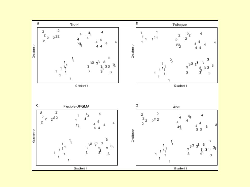
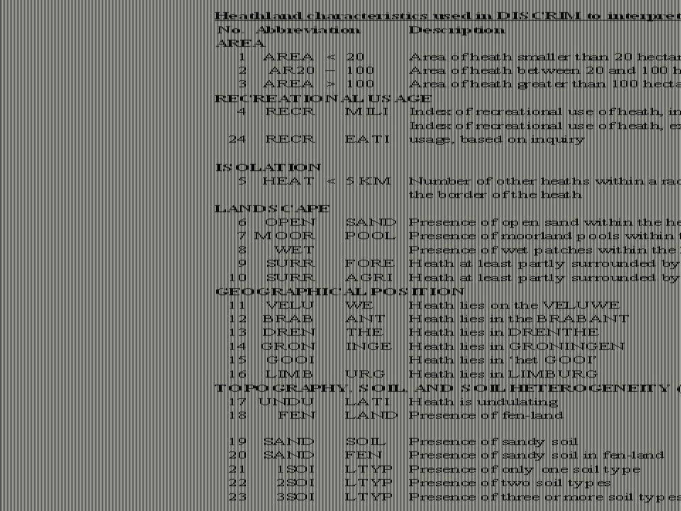


>")


.>")


