1. MHD vs. kinetic effects in space & solar plasmas
David Tsiklauri
University of Salford
STFC Introductory
Summer School in Solar & Solar-Terrestrial Physics
12 September 2007  
Armagh Observatory

2. Different types of plasma description / Lecture outline:
1. Fluid / MHD description
2. Dynamics of individual particles
3. Kinetic (statistical approach)
4. Applications (to space plasmas: waves + reconnection)
1. Fluid / MHD description:
In this approach plasma is described in terms of macro-parameters
such as density, pressure and velocity of "physically small" fluid
volume elements that contain many plasma particles.
Such description is justified if there is a certain ordering of spatial &
temporal scales in the physical system. A priori such ordering is not
clear from the MHD equations. What is clear is that these equations
are invalid when λ (wavelength) is too small and ω (frequency) is
too large [spatial scale= SS and temporal scales = TS]

3. Neglecting charge separation immediately restricts rage of
applicability of the MHD with λ >> λD (Debye length)=
The assumption that ne= ni i.e. e's & i's move together puts yet
another restriction on TS's of MHD processes, namely, T >> ωci-1 .
This inequality follows from the fact that for such fast rotation as
cyclotron, e's & i's move differently. (ωci =eB/mic – IC frequency)
MHD also neglects tensor nature of thermal pressure:
This assumption would clearly hold if collisions play dominant role.
However, on TS smaller than collision time this is not the case.
In MHD, in addition to λ >> λD , and following ordering should hold
(Roberts & Taylor (PRL, 1962 and references therein) :
(MHD ordering) (1.1)

4. In the situation when ordering between TS and SS of the system is
different other types of MHD are used. In particular, if
(FLR MHD ordering) (1.2)
the pressure tensor is even non-diagonal. In such, cases Finite Larmor
Radius (FLR) MHD is used (e.g. Berning & Spatschek PoP 1998):
They are closed by some kind of equation of state e.g. isothermal. The gyro-viscous pressure tensor can be found in (Hazeltine & Meiss, Plasma Confinement, 1991).
(1.3)

5. Other examples of MHD-type equations can be derived based of
which terms are significant (i.e. kept) in the generalized Ohm's law.
Recall that the simplest form of Ohm's law quoted on previous slide
is derived from following consideration:
Plasma is a moving conductor and the Ohm's law should be written in
the plasma rest frame For non-relativistic flows the rest
frame electric field is
Because of quasi-neutrality condition, we require j=j'. Thus, the
Ohm's law for (moving) plasma is:
(1.4)

6. Indeed, simple Ohm’s law, Eq. (1
Indeed, simple Ohm’s law, Eq.(1.4), takes into account fluid motion in the magnetic field (appearing as an additional electric field (V × B)/c) but not the effects due to the acceleration, dV /dt , of the plasma
fluid volumes (Polygiannakis & Moussas, Plasma Phys. Control. Fus. 43 (2001) 195).
In the non-inertial coordinate system co-moving with the flow, the acceleration appears as an inertial force −mdV /dt (where m is the ion mass, since the electrons are much lighter), thus corresponding to an ‘inertially’ exerted electric field −(m/e)(dV /dt).
Thus the generalized Ohm’s law must include the total electric field exerted on plasma volume (Landau & Lifshitz Electrodyn. Cont. Med, 1963, p 210):
(1.5)

7. If we insert dV /dt from the equation of plasma motion we obtain:
where n = ρ/m is the number density.
Note that Eq.(1.6) is an approximation of more extended expressions, obtained by taking into account both e's & i's equations of motion. However these terms are negligible in the usual MHD limit (e.g. Krall and Trivelpiece 1973).
(1.6)
In the generalized Ohm’s law (1.6) notice the additional Hall term, (J × B)/enc (for which the plasma model is often called Hall-MHD) and (tensor) pressure gradient, ∇Pth/en, electron inertia
and some other force (e.g. gravity), −F/en, terms.

8. The relative importance of the Hall term can be examined if writing
(1.6) as (e.g. see also Parks Physics of Space Plasmas. An Introd. 1991, p 278):
(1.7)
where
is the ‘total’ electric field without the Hall term;
is the electron gyrofrequency;
is the frequency of charge collisions (assuming that the conductivity is mainly due to electrons);
Then (1.7) shows that the Hall current, J × B/B, becomes dominant
over the ‘usual’ electric field-aligned current, J, if ωce >> ν which is
valid for the limiting case of strong magnetic fields or of rare
charge collisions.

9. Indeed, many astrophysical problems involve nearly collisionless plasmas (e.g. the solar wind), while confined plasma experiments involve plasmas embedded in strong magnetic fields.
Therefore, the Hall current in those cases is expected to be as much or even more important than the electric field-aligned current.
Let us make simple estimate for solar corona:
ωce = 1.76 ×107 B[G]= 1.76 ×109 rad s-1 (for 100 Gauss)
ν = (4.8 × 10-10)2 × 2. × 109/(9.1 × × 6. × 1016) ≈ 10 s-1 . Thus
ωce / ν ≈ 108 >> 1.
At the same time we should be aware that the importance of the Hall
term applies only on small scales, e.g. magnetic reconnection.
For details see Bhattacharjee, Annu. Rev. Astron. Astrophys , 365; Ma & Bhattacharjee (1996) Priest & Forbes (2000); and Birn et al., J. Geophys. Res., 106, 3715 (2001).

10. 2. Dynamics of individual particles
In this approach plasma is described in terms of the dynamics of
individual particles.
Plasma has natural tendency to disperse. This is due to the fact that
plasma particles move randomly in every direction (thermal motion).
Unless there is a restraining force, plasma will disperse & cease to exist.
One possibility is that particle collisions, which naturally tend to
deflect them from their ran-away trajectories could play role of the
restraining force.
However, in many plasmas, particularly space plasmas, collisions are
too rare, i.e. the collision frequency ν << other characteristic
frequencies of the system.
In such cases magnetic field, which acts via Lorentz force is far more
important than collisions as the restraining force.

11. The Lorentz force acting on a charge is:
If we only consider action of B-field on an electron (E-field is usually
ignored because it is of the order of V2/c2 <<1), then Newton's 2nd
law gives:
(2.1)
which after defining electron cyclotron frequency vector,
gives
(2.2)
In principle Eq.(2.2) can be solved (details in
e.g. R.O. Dendy, Plasma Dynamics, chapter 2)
and thus particle trajectory can be determined.
In a uniform magnetic field the path of an
electron is helical as shown in the figure →
The helix is produced by uniform circular
motion about a point that moves with
constant speed parallel to the magnetic field.

12. The electron position can be written as:
which implicitly defines the guiding centre (GC) position (see fig.→).
The first term on RHS describes the parallel dynamics, while the second clearly describes perpendicular dynamics
is the mean position of the electron if the rapid variation (rotation)
is averaged out. This means position and also (i.e. the
drift velocity of the GC) often contains all the information required,
which is useful when one wants to follow path of over a
timescale >> ωce-1.

13. Guiding Centre approximation.
In general, when B=B(r,t) then particle dynamics is rather complicated. However, when L >> rL,e and T >> ωce-1 (L and T are spatial and times scales of the magnetic field variation), the Guiding Centre approximation apples.
In this approach the helical trajectory of a particle in magnetic field is approximated by a smooth drift motion of the GC as depicted in this figure:
This speeds up numerics
e.g. Genot et al. (2004)
Ann. Geophys., 6, 2081

14. Let’s look at relation between some characteristic frequencies:
electron collision frequency νe, plasma frequency ,
and cyclotron frequency for solar corona and fusion
plasmas.
Parameters can be taken from e.g.
NRL plasma formulary:
Fusion plasmas n=1014cm-3 T=103eV
Solar corona n=109cm-3 T=102eV
(note 1eV=11600K) Hz Hz Hz
Here n [cm-3]; T [eV]; B in [G] and
Coulomb logarithm (for electrons) is

15. B. The Larmor radius is comparable to Debye radius:
fce Hz
fp Hz Hz
Fusion
2.8x1011
1011
1.4x105
Corona
2.8x108
3x108 53 e n
Two important
conclusions follow
from these estimates:
1. For the both cases fce/ νe ≈ few x106 which means that between every collision electrons rotate millions of times around magnetic field line. Thus for solar coronal and fusion plasma magnetic field plays far more important role as a restraining force than collisions.
2. For the both cases fce/ fe ≈ 1 which means that. This coincidence is responsible for a great degree of complexity in the plasma behaviour.
A. Mathematically this makes the dispersion relations become difficult to treat.
B. The Larmor radius is comparable to Debye radius:

16. 3. Kinetic (statistical approach)
In plasma kinetics instead of studying dynamics of individual particles,
without loss of generality, system is ascribed distribution function (DF)
fα(r,p,t) which is the probability of finding species α, in intervals
(r,r+dr) and (p,p+dp) at t=t. Hence, normalization condition should be:
Using this microscopic distribution function, macroscopic (i.e. hydro-
dynamic) quantities can be defined as n-th order moments :
(3.1) 0-th order
(3.2) 1-st order
i.e. 0-th order gives number density,
1st order gives definition of the hydrodynamic velocity Vα.
Here we will consider non-relativistic case i.e. pi=mvi,
Also the following notation is used throughout:

17. 2-nd order moment allows to define the pressure tensor pij:
(3.3)
Vlasov equation
Let us derive equation which governs dynamics of the distribution
function – with the latter, we can construct all the quantities we need.
If plasma is rarefied (particle collisions can be ignored) and particles
are not created or annihilated, then all we need to require is that the DF
does not change in time:
which is the same as:
(3.4)

18. In principle any force can be put in Eq. (3
In principle any force can be put in Eq.(3.4), but for plasma, which is a
collection of charged particles, and the strongest force acting is of EM
nature, it has to be the Lorentz force:
(3.5)
When E(r,t) and B(r,t) EM-fields are determined from the Maxwell's
equations in which instead of charge and current densities ρq and j
the following equations are used: and ,
then eq.(3.5) is called Vlasov's equation with self-consistent EM fields.
Self-consistent in the sense that, Eq.(3.5) provides DF, fα, which
changes under the effect of EM-fields. In turn, change in DF means
re-distribution of charges, i.e. change in EM-fields; or in one line:
EM-fields affect DF, which in turn affects EM-fields in a
self-consistent way.

19. We have seen how taking different order moments of the DF gives
different macroscopic quantities. Now, we will show how taking different order moments of the Vlasov's equation gives different
conservation laws (mass, momentum, energy, etc.).
Let us take 0-th order moment of Eq.(3.5): =0
which after multiplying by mα and noting that ρα= mα nα we obtain
Eq.(3.6) is mass conservation (continuity) equation for species α. Familiar single fluid MHD version of Eq.(3.6) can be obtained by:
(3.6)
mass, charge, current densities, hydrodynamic velocity

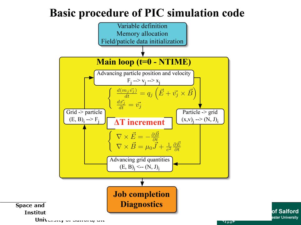
20. 4. Applications (to space plasmas: waves + reconnection)
Previously we discussed charged particle dynamics. In principle,
plasma dynamics can be described by solving the equation of motion
for each individual particle (initially distributed by e.g. Maxwell
distribution), supplemented by the Maxwell's equations in which
charge and current densities are determined self-consistently i.e. by
summing the spatially and temporally changing distribution of plasma
charged particles.
This type of approach is called Particle-In-Cell (PIC) simulation.
Typically 100s of millions of particles are used, i.e. above mentioned
equations are solved for each of the 100s of millions of particles!

21. This may sound complicated, but it is still better than tackling
Vlasov's equations in 6D (3V, 3D) space: consider memory constraints:
if one doubles the resolution then need 26=64 times more RAM!
PIC has shortcomings too: it is hard to properly resolve high velocity
tails of the distribution function: if you typically have 100 particles per
cell at v = vth than for v >> vth, there are only few particles left (poor
statistics). Also, PIC data is usually quite noisy – needs smoothing.
In PIC simulation EM-fields are defined on some spatial grid
(i.e. are discrete variables), while particle positions are continuous.
Particles start to move under Lorentz force, hence charge distribution
changes; this changes EM-fields (which are calculated using
Maxwell's equations in which charge and current densities are
determined self-consistently), and so on.

23. Particle-in-cell simulations of circularly polarized Alfven wave
(AW) phase mixing: What is Phase Mixing?
Phase Mixing is a mechanism originally proposed by Heyvaerts &
Priest (1983) that suggests that AW dissipation in plasmas with
inhomogeneity across the magnetic field is greatly enhanced:
Classical (resistivity) dissipation:
Phase Mixing (enhanced) dissip.:
All previous Phase Mixing studies were performed in MHD
approximation (Heyvaerts & Priest 1983; Nocera et al. 1986; Parker
1991; Nakariakov et al. 1997; DeMoortel et al. 2000; Botha et al.
2000; Tsiklauri et al. 2001, 2002, 2003; Hood et al. 2002; Tsiklauri &
Nakariakov 2002).

24. The problem with this, of course, is that MHD approximation
will eventually break down: First when transverse scale in a wave
front will reach ion gyro-radius, ri, and then the electron one, re.
Hence we decided to perform Particle-in-cell i.e. kinetic simulations
of circularly polarized AW phase mixing for the first time.
The results are published in two papers:
Tsiklauri D. , J.-I. Sakai, S. Saito,
Astron. Astrophys., 435, 1105, (2005).
New J. Phys., 7, 79, (2005).
What was new to expect?
Ability to study wave—
particle interactions!
How “dissipation”
(collisionless) is modified
in the kinetic regime!
What happens to individual
species (electrons and ions)?

25. Key facts about PIC simulations of Alfven wave phase mixing:
We use 2D 3V fully relativistic, electromagnetic, PIC code.
System size Lx=5000Δ by Ly=200Δ cells.
Each cell has 100 electrons and ions. Total of 478 x 106 particles!
Plasma density is enhanced by a factor of 4 in the middle of simulation domain:
Temperatures and therm. speeds of e,i are varied so that ptot=const.
Mass ratio used: mi / me = 16.
Alfven wave phase mixing takes place.
Dissipation of Alfven waves is greatly enhanced due to wave-particle interactions (as shown in the following slides).

26. Simulation results: Alfven wave dynamics ...
t = 16ωci
t = 31ωci
t = 55ωci

27. Developed
stage of
Phase-Mixing
t = 55ωci.
Not
Phase-
Mixed AW
comps.
By and Ez
Phase-Mixed AW
components
Bz and Ey
N.L.
generated Bx
N.L.
generated
electron
density

28. Simulation results: Evidence of electron acceleration
Electric field that accelerates electrons
Electr. Phase Space (Vx vs x) and (Vx vs y)

29. What about particle distribution functions?
Vx, Vy, Vz –
distribution
functions of
electrons
(top row)
and ions
(bottom row)
at t = 0
(dotted
curves) and
t = 55/ωci
(solid curves).
Electron
accleration
Ion wave-
broadening

30. What about AW amplitude decay law?
Two snapshots of the AW Bz(x, y = 148)
component at t = 54.69/ωci (solid line)
and t = 46.87/ωci (dotted line).
The dashed line represents fit
0.056 exp[− (x/1250)3].
This nicely reproduces
Heyvaerts & Priest (1983) result!
i.e. our kinetic simulations recovered
MHD AW amplitude decay law:
Also, measured AW speed (by the two
snapshots) corresponds to the bumps
in the electron distribution function!

31. Ok, so what we've learned: if one drives Alfven (IC) waves (0.3ωci) in
plasma with transverse density inhomogeneity then E|| is generated ...
What is the essential physics? or a minimal model which can do the job?
It turns out [see Tsiklauri, New J. Phys. 9, 262 (2007)] that a two fluid
model (which allows for electron and ion separate dynamics) can do it!
Here mi/me=262, takes 4 days on 1 CPU – equivalent PIC simulation
would have taken 4 month on 64 CPUs!
E||=100Vm-1

32. Magnetic reconnection is one of important possible ways of
Magnetic reconnection during collisionless, stressed, X-point collapse using Particle-in-Cell simulation
Magnetic reconnection is one
of important possible ways of
converting magnetic field
energy into heat and accelerated
plasma particles.
Main problem in plasma
heating (solar corona,
Tokamak) is that
Spitzer resistivity is ~ T -3/2,
i.e. more heating =
plasma starts to behave
as a superconductor.
resistive (collisional)
or collisionless
spontaneous or
forced
steady
timedependent
reconnection
Main aspects of reconnection
can be classified as:

33. Resistive reconnection of all said types is very well studied (e. g
Resistive reconnection of all said types is very well studied (e.g. Priest
& Forbes book, CUP 2000), although there are some open questions,
particularly in 3D. Collisionless reconnection is a relatively recent
development (e.g. Birn & Priest book, CUP 2007, chapter 3.1, Fig.3.1)
The key question is which term
in the generalized Ohm's law is
breaking the frozen-in condition?
Each term has different spatial
scales associated with it:
For electron inertia – c/ωpe – electron skin-depth;
For the Hall term – c/ωpi – ion skin-depth;
For the pressure tensor – rLi – ion Larmor radius;

34. Validation of our PIC (Particle-In-Cell) code by reproduction of
GEM challenge results
General Advice:
Always try to reproduce previous results when using a new code or
using an old code for a new application!
GEM result
[Pritchett, JGR, 106, 3783, (2001)]
Our result
Time evolution of the reconnected magnetic flux difference, Δψ

35. Magnetic reconnection during collisionless, stressed, X-point
collapse using Particle-in-Cell simulation
For details see Tsiklauri & Haruki, PoP (accepted)
Solar flare model
Our equivalent numerical simulation
(Hirayama 1974)
a = 1
a > 1
Aschwanden “Physics of
the Solar corona An Introduction”
Priest & Forbes “Magnetic Reconnection
MHD Theory & Applications”

36. The model
Magnetic field:
Parameters:
Lx = Ly = 400D (lD = 1D)
wpe Dt = 0.05
N = 1.6 million e-i pairs (n0 = 100 / cell)
L = 200D
c/wpe = 10D
mi / me = 100
vte / c = 0.1
wce/wpe = 1.0 (for B = B0 )
Imposed current:
b = 0.02
vd / c = (a = 1.2)
Boundary conditions (this is crucial):
E and B fields – No flux trough boundary
Particles Reflection

37. Generation of out-of-plane electric field
Out-of-plane electric field in the X-point (magnetic null) vs time. This
field is a measure of magnetic reconnection.
wpet = 250 corresponds to 1.25 (Alfven times)

38. Current sheet generation
Time evolution
of spatial
distribution of
total current
jz in the X-Y
plane.
Note the current
peaks at the same
time as Ez
(on previous
slide)
wpet = 0
100
Y / (c/wpe)
X / (c/wpe)
170
250
jz / j0
Max (jz / j0) = 16

39. Generation of Quadruple out-of-plane magnetic field
Time evolution Bz in the X-Y plane
Such field is
regarded as
evidence for
Hall effect
physics –
separation
of electron
and ion flow.
[e.g. Birn, et al.,
JGR, 106, 3715
(2001);
Uzdensky &
Kulsrud, PoP,
13, 2305 (2006)]
wpet = 0
100
Y / (c/wpe)
X / (c/wpe)
170
250
Bz / B0

40. Visualization of magnetic reconnection by tracing dynamics of
individual magnetic field lines:
| B | / B0 =
1.55, 1.60,
1.65, 1.70 y x

41. Particle acceleration in the current sheet
The local electron energy spectrum (distribution function) near the current sheet at t = 0 (dashed curve) and t = 250 (solid curve) for α= 1.20.
Fit (solid straight line) to
the high energy part
of the spectrum shows a
clear power law:
In the vicinity of X-type
region in the Earth's
magneto-tail observations
show power law index is
between -4.8 and -5.3
[Oieroset, et al., PRL 89, , (2002)]

42. Separation of electron and ion flow in the current sheet
Electron inflow (a) concentrated along the separatrices. They deflect from the current sheet on the scale of electron skin depth, with the electron outflow speeds being ≈ the external Alfven speed 0.13c.
Ion inflow (b) starts
to deflect from the
current sheet on
ion skin depth
scale [10(c/ωpe)].
Outflow speeds ≈0.03c.
Task: read chapter 3.1
from Birn & Priest 2007
book and compare
these to their Fig. 3.1
(slide 33)

43. Energetics of the reconnection process
One of the main problems in
solar physics is the time scale
of energy release during solar
flares:
Normal resistive time is:
1015 Alfven times (108 yr)
Flares typical time is:
Alfven times!
In our simulation of x-point
collapse up to 20% of initial
magnetic energy is
released in just
one Alfven time!