Download presentation
Presentation is loading. Please wait.

1
Finance and the Financial Manager
Chapter 1

2
1.2 The Role of the Financial Manager
1.1 What is a Corporation? 1.2 The Role of the Financial Manager Two Basic Questions Investment Decision 1 Financing Decision 2

3
1.3 Who is the Financial Manager
(2) (1) Financial Firm's Financial (4a) Manager Operations Markets (3) (4b)
 (1) Financial. Firm s. Financial. (4a) Manager. Operations. Markets. (3) (4b)")
4
1.4 Goal of the Firm ?

5
1.5 Agency Problem A. Separation between Ownership and Management
B. How to solve agency problem? Monitoring by board of directors 1 Compensation package 2 Monitoring by outside large blockholders (Bank, insurance Co., pension, mutual fund) 3 Efficient outside managerial labor market 4 Active outside takeover market 5
 3. Efficient outside managerial labor market. 4. Active outside takeover market. 5.")
6
Present Value and The Opportunity Cost of Capital
Chapter 2

7
2.1 Introduction A. Present Value B. Risk and Present Value
PV = C / (1+r) r: NPV = PV - C0 B. Risk and Present Value C. PV and Rate of Return
 r: NPV = PV - C0. B. Risk and Present Value. C. PV and Rate of Return.")
8
D. The Opportunity Cost of Capital
From your Investment 1 C0 : $ 100,000 C1 : Slump : $ 80,000 Normal : $ 110,000 Boom : $ 140,000 E(C1)
")
9
Find stock X which has same risk as your project :
From Stock Market 2 Find stock X which has same risk as your project : P0 : $ 95.65 P1 : Slump : $ 80 Normal : $ 110 Boom : $ 140 E(P1) = 1/3 ( ) = 110 E(R) = = 0.15 15% k 95.65
 = 1/3 ( ) = 110. E(R) = = 0.15 15% k ")
10
Q : What is the Present Value of your project?
PV of project = NPV =

11
How to Calculate Present Values
Chapter 3

12
3.1 Cash Flows in Several Periods (*)
3.2 Perpetuities and Annuities (*) 3.3 Growing Perpetuities (*) 3.4 Compounding Interest (*)
 3.3 Growing Perpetuities (*) 3.4 Compounding Interest (*)")
13
3.5 Nominal and Real Interest
A. Real CF = Nominal CF (1+inflation rate) (1+ Nominal rate) (1+inflation rate) B. (1+Real Rate) = 3.6 Bond Valuation C 1+r C (1+r)2 C+F (1+r)n … ... PVbond = + + + = C PVAF + F PVF (Ex) Coupon rate: 10%, r=5%, face value=$1,000 N=7years PVbond = 100 = $1360.7
 (1+ Nominal rate) (1+inflation rate) B. (1+Real Rate) = 3.6 Bond Valuation. C. 1+r. C. (1+r)2. C+F. (1+r)n. … ... PVbond = = C PVAF. + F PVF. (Ex) Coupon rate: 10%, r=5%, face value=$1,000 N=7years. PVbond = 100 = $")
14
The Value of Common Stocks
Chapter 4

15
4.1 How Common Stocks are Traded?
A. Primary Market B. Secondary Market NYSE AMEX OTC (NASDAQ)
")
16
4.2 Stock Valuation + A. Today’s Price
E(R) = (P1 - P0 + DIV) / P0 = r r: market capitalization rate P1 - P0 P0 DIV + = = Holding Period Return = E(R) (Ex) P0 = $100 , P1 = $110 , DIV = $5 r =
 = (P1 - P0 + DIV) / P0 = r. r: market capitalization rate. P1 - P0. P0. DIV. + = = Holding Period Return = E(R) (Ex) P0 = $100 , P1 = $110 , DIV = $5. r =")
17
P0 = (P1 + DIV) / (1+r) = ( ) / 1.15 = 100 $ 100 ; equilibrium price if 15% is an appropriate discount rate Q: What happen if P0 is different from $100 ?

18
B. What determines next year’s price ?
Valuation Model P0 = (P1 + D1) / (1 + r), P1 = (P2 + D2) / (1 + r) P0 = D1 / (1 + r) + (P2 + D2) / (1 + r)2 = D1 / (1 + r ) + D2 / (1+r)2 + D3 / (1 + r)3 + ……… = t=1 Dt / (1 + r)t Assume: Dividend grows at a constant rate; g P0 = [D0 • (1 + g)] / (r - g) = D1 / (r - g)
 / (1 + r), P1 = (P2 + D2) / (1 + r) P0 = D1 / (1 + r) + (P2 + D2) / (1 + r)2. = D1 / (1 + r ) + D2 / (1+r)2. + D3 / (1 + r)3 + ……… = t=1. Dt / (1 + r)t. Assume: Dividend grows at a constant rate; g. P0 = [D0 • (1 + g)] / (r - g) = D1 / (r - g)")
19
EX : Pinacle West Corp (p 69)
4.3 Simple Way to Estimate r r = D1 / P0 + g D1 / P0 : Dividend Yield g : Dividend Growth EX : Pinacle West Corp (p 69) P0 = $41, Div1 = $1.27, g = 5.7% r =
 P0 = $41, Div1 = $1.27, g = 5.7% r =")
20
r = 0.031 + 0.053 = 0.084 or 8.4% Alternative Approach:
Payout ratio = DIV1 / EPS = 0.47 Plowback Ratio = 1- Payout ratio = 0.53 ROE = EPS / Book Equity per Share = 0.1 g = Plowback ratio * ROE = r = = or 8.4%

21
Some Warnings about Constant-Growth Formulas
1. Individual stock’s r is subject to estimation errors Portfolio approach 2. Growth rate can rarely sustained indefinitely Ex. Growth-tech DIV1=$0.05, P0=$50, Plowback Ratio=80%, ROE=25% g = r =

22
Ex: at t=3 and thereafter ROE =16%
Firm responds by plowing back 50% of earnings g = Table 4.2 YEAR1 YEAR2 YEAR3 YEAR4 Book equity 10.00 12.00 14.40 15.50 Earning per share, EPS 2.50 3.00 2.30 2.49 Return on Equity, ROE .25 .25 .16 .16 Payout ratio .20 .20 .50 .50 Dividends per share, DIV .50 .60 1.15 1.24 Growth rate of dividends - .20 .92 .08

23
General DCF formula to find the capitalization rate r:
DIV1 1+r DIV2 (1+r)2 DIV3 + P3 (1+r)3 P0 = + + P3 = P0 = 50 =
2. DIV3 + P3. (1+r)3. P0. = + + P3. = P0. = 50. =")
24
Growth stock vs Income stock
4.4 The link between stock price and earning per Share Growth stock vs Income stock A. Income Stock No Growth Perpetuity Model EPS1 r DIV1 P0 = = r (EX) Expected Return = Dividend Yield = 10/100 =.10 = r Price = DIV1 / r = EPS1 / r =
 Expected Return = Dividend Yield = 10/100 =.10 = r. Price = DIV1 / r = EPS1 / r =")
25
B. Growth Stock (r=10%) at t = 1: (once & for all)
Invest $10 into project with permanent return of 10% $ 1 (each year) NPV = This investment contributes “0” to value. (EX) Return on project is higher or lower than 10%; NPV? (go to table 4-3)
 NPV = This investment contributes 0 to value. (EX) Return on project is higher or lower than 10%; NPV (go to table 4-3)")
26
Table 4-3 Effect on stock price investing an additional $10 in year 1 at different rates of return. Notice that the earnings-price ratio overestimates r when the project has negative NPV and underestimates it when the project has positive NPV. Project's impact Project Rate Incremental Project NPV Share Price EPS1 on Share Price a in Year 0, P0 of Return Cash Flow, C in Year 1 in Year 0 b P r .05 $ .50 - $ 5.00 - $ 4.55 $ .105 .10 .10 1.00 100.00 .10 .10 .15 1.50 104.55 .096 .10 .20 2.00 109.09 .092 .10 .25 2.50 113.64 .088 .10 a Project costs $ (EPS1). NPV = C / r, where r = .10 b NPV is calculated at year 1. To find the impact on P0, discount for 1 year at r = .10
. NPV = C / r, where r = .10. b. NPV is calculated at year 1. To find the impact on P0, discount for 1 year at r = .10.")
27
In general : r P0 = + PVGO r :
EPS1 r P0 = + PVGO PVGO : Present Value of Grow Opportunity Sum of all NPVs (per share) EPS1 r Capitalized value of average earning under a no-growth policy :
 EPS1. r. Capitalized value of average earning. under a no-growth policy. :")
28
Is Japanese firm growing fast?
Determinants of P/E Ratio P0 = PVGO EPS1 r + Divide each side by EPS P/E = 1 r PVGO E + 1. Cost of Capital(r): “-” 2. Conservative accounting procedure(EPS): “-” 3. Growth opportunities(PVGO): “+” Q : Japanese firm : P/E 50 U.S. firm : P/E 17 Is Japanese firm growing fast?
: - 2. Conservative accounting procedure(EPS): - 3. Growth opportunities(PVGO): + Q : Japanese firm : P/E 50. U.S. firm : P/E 17. Is Japanese firm growing fast")
29
EX : Fledgling Electronics Case (p73)
r = 15 % , D1 = $ 5 P0 = D1 / (r - g) = If EPS1 = $ 8.33, Payout ratio = D1 / EPS1 = 5 / 8.33 = 0.6 If ROE = .25, g = P0 =
 = If EPS1 = $ 8.33, Payout ratio = D1 / EPS1 = 5 / 8.33 = 0.6. If ROE = .25, g = P0 =")
30
Analyze: $ 44.44 Plowback Ratio = .4, * .4 = $ 3.33 Invest: $ 3.33 at 25% (ROE) .25 * 3.33 = $ .83 at t = 1; NPV1 = / .15 = 2.22 at t = 2; Invest 3.33 * 1.1 = 3.69 (g = 10%) NPV2 = * (.83 * 1.1) / .15 = 2.44 PVGO = NPV1 / (r - g) = 2.22 / ( ) = $ 44.44 This is growth stock, not because g = 10%, but because
 NPV2 = * (.83 * 1.1) / .15 = PVGO = NPV1 / (r - g) = 2.22 / ( ) = $ This is growth stock, not because g = 10%, but because.")
31
C. Some Example of Growth Opportunities
Table 4-4 Estimated PVGOs (p.76) Market PVGO, Stock Capitalization PVGO Percent of Price, P0 EPS* Rate, r** =P0 - EPS/r Stock Price P / E Income Stocks: AT & T $52.00 $2.85 .094 $21.70 41.7 18.2 Conagra 26.00 1.33 .106 13.50 51.7 19.5 Duke Power 60.00 3.58 21.90 36.5 16.8 Exxon 64.00 2.89 .099 34.70 54.3 22.1 Growth Stocks: Compaq 30.00 0.69 .123 24.40 81.3 43.5 Merck 120.00 4.43 .118 82.50 68.7 27.1 Microsoft 101.00 2.08 .165 85.10 84.2 48.6 Wal-Mart 0.73 52.20 87.1 82.2 * EPS defined as the average earnings under a no-growth policy. As an estimate of EPS, we use the forecasted earnings per share for the 12 months ending March31, Source: Value Line. * The market capitalization rate was estimated using the capital asset pricing model. We describe this model and how to use it in Section 8.2 and EX: market risk premium = 6%
 Market. PVGO, Stock. Capitalization. PVGO. Percent of. Price, P0. EPS* Rate, r** =P0 - EPS/r. Stock Price. P / E. Income Stocks: AT & T. $ $ $ Conagra Duke Power Exxon Growth Stocks: Compaq Merck Microsoft Wal-Mart * EPS defined as the average earnings under a no-growth policy. As an estimate of EPS, we use the forecasted. earnings per share for the 12 months ending March31, Source: Value Line. * The market capitalization rate was estimated using the capital asset pricing model. We describe this model and how to use it in Section 8.2 and 9.2. EX: market risk premium = 6%")
32
Why NPV leads to better Investment Decisions than Other Criteria
Why Net Present Value Leads to Better Investment Decisions than Other Criteria Chapter 5

33
5.1 Review of Basics Forecast Cash Flow
2 Determine appropriate Cost of Capital 3 Discount with Cost of Capital

34
All cash flows are considered
Q : Why NPV ? All cash flows are considered Time Value of Money NPV is not affected by manager’s taste, accounting method, profitability of existing business, and profitability of other independent business

35
5.2 Payback Period Number of years it takes before cumulative
cash flow recovers initial investment CASH FLOWS, DOLLARS Payback NPV at Project C0 C1 C2 C3 Period, Years 10 Percent B - 2,000 + 500 + 5,000 3 2,642 C - 2,000 500 +1,800 + 5,000 2 -58 D - 2,000 + 1,800 2 +50

36
Cash flow vs. Book Income
5.3 Book Rate of Return Book income Book Rate of Return = Book assets Cash flow vs. Book Income Problems :

37
Example Computing the average book rate of return on an investment of $9000 in project A CASH FLOWS, DOLLARS Project A Year 1 Year 2 Year 3 Revenue 12,000 10,000 8,000 Out-of-Pocket cost 6,000 5,000 4,000 Cash flow 6,000 5,000 4,000 Depreciation 3,000 3,000 3,000 Net income 3,000 2,000 1,000 average annual income 2,000 Average book rate of return = = = .44 average annual investment 4,500 Year 0 Year 1 Year 2 Year 3 Gross book value of investment $ 9,000 $ 9,000 $ 9,000 $ 9,000 Accumulated depreciation 3,000 6,000 9,000 Net book value of investment $ 9,000 $ 6,000 $ 3,000 $ Average net book value = $ 4,500

38
5-3 Internal Rate of Return: IRR
Discount rate that makes NPV = 0 C0 = - 4, k: cost of capital C1 = 2,000 C2 = 4,000 NPV = -4,000 + (1+IRR) 2,000 + 4,000 (1+IRR)2 = 0 (Rule) Accept IRR>k NPV>0 Reject IRR<k NPV<0
 2, ,000. (1+IRR)2. = 0. (Rule) Accept IRR>k NPV>0. Reject IRR<k NPV<0.")
39
Net Present Value, dollars
2500 2000 1500 IRR=28% 1000 500 10 20 30 40 50 60 70 80 90 100 -500 Discount rate (%) -1000 -1500 -2000
")
40
Pitfall 1. Lending vs. Borrowing?
CASH FLOWS, DOLLARS NPV at Project C0 C1 IRR, Percent 10 Percent A - 1,000 + 1,500 + 50 B + 1,000 - 1,500 CASH FLOWS, DOLLARS NPV at Project C0 C1 C2 C3 IRR, Percent 10 Percent C + 1,000 - 3,600 + 4,320 - 1,728 + 20 - .75

41
60 40 20 -20 10 Discount rate (%) Net Present Value, dollars 30 50 80
20 40 60 10 Discount rate (%) Net Present Value, dollars 30 50 80 90 100 70
 Net Present Value, dollars")
42
Pitfall 2. Multiple Rates or Return
1 2 3 4 5 6 Pretax -1,000 300 300 300 300 300 300 +500 -150 -150 -150 -150 -150 Tax Net -1,000 800 150 150 150 150 -150 CASH FLOWS, DOLLARS NPV at Project C0 C1 C2 IRR, Percent 10 Percent D + 1,000 - 3,000 + 2,500 none + 339

43
1000 NPV 500 -500 -1000 Discount Rate IRR=15.2% IRR=-50%

44
Pitfall 3. Mutually Exclusive Projects
3.1 Different scale CASH FLOWS, DOLLARS NPV at Project C0 C1 IRR, Percent 10 Percent E - 10,000 + 20,000 100 F - 20,000 + 35,000 75 CASH FLOWS, DOLLARS NPV at Project C0 C1 IRR, Percent 10 Percent F-E - 10,000 + 15,000 50 + 3,636

45
3.2 Different pattern of cash flow over time
CASH FLOWS, DOLLARS IRR, NPV at Project C0 C1 C2 C3 C4 C5 Etc. Percent 10 Percent G - 9,000 +6,000 +5,000 +4,000 … 33 3,592 H - 9,000 +1,800 +1,800 +1,800 +1,800 +1,800 … 20 9,000 I -6,000 +1,200 +1,200 +1,200 +1,200 … 20 6,000

46
10,000 NPV, dollars -5000 Discount Rate, percent 33.3 15.6 +5,000 +6,000 10 20 30 40 50 Project G Project H

47
Pitfall 4. What happens if term structure is not flat?
(generally) NPV = - C0 + C1 / (1+r1) + C2 / (1+r2)2 + … IRR vs r1 r ? r3
 NPV = - C0 + C1 / (1+r1) + C2 / (1+r2)2 + … IRR vs. r1. r2 r3.")
48
5.5 Limited Resource (Capital Rationing)
CASH FLOWS, MILLIONS OF DOLLARS NPV at Project C 1 2 10 Percent A - 10 + 30 + 5 21 B - 5 + 20 16 + 15 12

49
<$10> t=0, t=1 NPV at Profitability Project C 10 Percent Index A
CASH FLOWS, MILLIONS OF DOLLARS NPV at Profitability Project C 1 2 10 Percent Index A - 10 + 30 + 5 21 2.1 B - 5 + 20 16 3.2 + 15 12 2.4 D - 40 + 60 13 0.4

50
More Elaborate Capital Rationing Models We accept proportion A of project A.
NPV of accepting A of A Previous Example NPV =

51
Constraint: (Costs) at t = 0, 10 A + 5 B + 5 C + 0 D 10 at t = 1, 40 D 30A + 5 B + 5 C + 10 0 A , B , C , D 1 Maximize: 21 A + 16 B + 12 C + 13 D Subject to : 10 A + 5 B + 5 C + 0 D 10 -30 A - 5 B - 5 C + 40 D 10

52
Making Investment Decisions with the Net Present Value Rule
Chapter 6

53
How to apply the rule to practical investment problems?
Question What should be discounted? CF: relevance, completeness, consistency, accuracy How NPV rule should be used when there are project interactions?

54
Estimate Cash Flow on an Incremental Basis
Average vs. incremental Include all incidental effects Do not forget NWC requirement Forget sunk cost Include opportunity costs Beware of allocated overhead costs Consider spillover effect “erosion”

55
(Ex) C0 C1 C2 C3 Treat Inflation consistently.
Real CF : discount with real rate Nominal CF: discount with nominal rate (Ex) C C C C3 Real CF rN = 15%, I = 10% NPV = NPV =
 C0 C1 C2 C3. Real CF rN = 15%, I = 10% NPV = NPV =")
56
6.2 Example - IMFC Project Initial investment: $ 10 mil
Salvage value at year 7: $ 1 mil (sold) Depreciation: 6 year straight line with arbitrary salvage of : $ 500,000 annual depreciation = = $ mil 9.5 mil 6
 Depreciation: 6 year straight line with arbitrary salvage of : $ 500,000. annual depreciation = = $ mil. 9.5 mil. 6.")
57
Table 6 - 1 Nominal Cashflow
Ex: forecast of inflation: 10% IM&C's guano project - revised projections reflecting (figures in thousands of dollars) PERIOD 1 2 3 4 5 6 7 1. Capital investment 10,000 -1,949* 2. Accumulated depreciation 1,583 3,167 4,750 6,333 7,917 9,500 3. Year-end book value 8,417 6,833 5,250 3,667 2,083 500 4. Working capital 550 1,289 3,261 4,890 3,583 2,002 5. Total book value (3 + 4) 8,967 8,122 8,511 8,557 5,666 2,502 6. Sales 523 12,877 32,610 48,901 35,834 19,717 7. Cost of goods sold 837 7,729 19,552 29,345 21,492 11,830 8. Other costs ** 4,000 2,200 1,210 1,331 1,464 1,611 1,772 9. Depreciation 10. Pretax profit ( ) -4,000 -4,097 2,365 10,144 16,509 11,148 4,532 1,449** 11. Tax at 35% -1,400 -1,434 828 3,550 5,778 3,902 1,586 507 12. Profit after tax -2,600 -2,663 1,537 6,594 10,731 7,246 2,946 942 * Salvage value. ** The difference between the salvage value and the ending book value of $ 500 is a taxable profit
 PERIOD Capital investment. 10, ,949* 2. Accumulated. depreciation. 1,583. 3,167. 4,750. 6,333. 7,917. 9, Year-end book value. 8,417. 6,833. 5,250. 3,667. 2, Working capital ,289. 3,261. 4,890. 3,583. 2, Total book value. (3 + 4) 8,967. 8,122. 8,511. 8,557. 5,666. 2, Sales , , , , , Cost of goods sold , , , , , Other costs ** 4,000. 2,200. 1,210. 1,331. 1,464. 1,611. 1, Depreciation. 10. Pretax profit. ( ) -4, ,097. 2, , , ,148. 4,532. 1,449** 11. Tax at 35% -1, , ,550. 5,778. 3,902. 1, Profit after tax. -2, ,663. 1,537. 6, ,731. 7,246. 2, * Salvage value. ** The difference between the salvage value and the ending book value of $ 500 is a taxable profit.")
58
IM&G’s guano project-cash-flow analysis
(thousand) Period 1 2 3 4 5 6 7 523 12,887 32,610 48,901 35,834 19,717 1. Sales 2. Cost of goods and sold 3. Other costs 4. Tax on operations 5. Cash flow from operation 6. Change in working capital 7. Capital investment and Disposal 8. Net cash flow 9. Present value at 20% Net present value = +3,519(sum of 9) 837 7,729 19,552 29,345 21,492 11,830 4,000 2,200 1,210 1,331 1,464 1,611 1,772 -1,400 -1,434 828 3,550 5,778 3,902 1,586 -2,600 -1,080 3,120 8,177 12,314 8,829 4,529 -739 -1,972 -1,629 1,307 1,581 2,002 -550 -10,000 1,442 -12,600 -1,630 2,381 6,205 10,685 10,136 6,110 3,444 -12,600 -1,358 1,654 3,591 5,153 4,074 2,046 961
 Period , , , , , Sales. 2. Cost of goods and sold. 3. Other costs. 4. Tax on operations. 5. Cash flow from. operation. 6. Change in working. capital. 7. Capital investment and. Disposal. 8. Net cash flow. 9. Present value at 20% Net present value = +3,519(sum of 9) , , , , ,830. 4,000. 2,200. 1,210. 1,331. 1,464. 1,611. 1, , , ,550. 5,778. 3,902. 1, , ,080. 3,120. 8, ,314. 8,829. 4, , ,629. 1,307. 1,581. 2, ,000. 1, , ,630. 2,381. 6, , ,136. 6,110. 3, , ,358. 1,654. 3,591. 5,153. 4,074. 2,")
59
Cash flow = Sales - CGS - Other costs - Taxes
Net cash flow = Cash flow from operation Networking capital [- Initial Investment + Recovery of Salvage Value] NPV =

60
Choosing between Long & Short Equipment
6.3 Project Interacting Choosing between Long & Short Equipment C0 C1 C2 C3 PV at 6% A +15 +5 +5 +5 28.37 B +10 +6 +6 21.00

61
Equivalent Annual Cost
PV at 6% Machine A +15 +5 +5 +5 28.37 EACA x x x 28.37 Machine B +10 +6 +6 21.00 EACB y y 21.00

62
Risk, Return & opportunity
Cost of Capital Risk and Return & Opportunity Cost of Capital Chapter 7&8

63
7.1 Seventy-Two year of Capital Market
Dollars 0.1 10 1000 1925 1933 1941 1949 1957 1965 1973 1981 1989 1997 5,520 Small Cap 1,828 S&P Corporate Bonds 39.07Government Bonds 14.25 Treasury Bills

64
Dollars 613.5 Small firms 203.2 S&P 500 6.16 Corporate bonds
0.1 10 1000 1925 1933 1941 1949 1957 1965 1973 1981 1989 1997 Small firms S&P 500 Corporate bonds Government bonds Treasury bills

65
Average rate of return on Treasury bills, Government bonds,
Corporate bonds, and common stocks, (Percent per year) AVERAGE ANNUAL RATE OR RETURN AVERAGE RISK PREMIUM (EXTRA RETURN VS. TRESURY BILLS) PORTFOLIO NOMINAL REAL Treasury bills 3.8 .7 Government bonds 5.6 2.6 1.8 Corporate bonds 6.1 3.0 2.3 Common stocks (S&P 500) 13.0 9.7 9.2 Small firm common stock 17.7 14.2 13.9
 AVERAGE ANNUAL. RATE OR RETURN. AVERAGE RISK PREMIUM. (EXTRA RETURN VS. TRESURY BILLS) PORTFOLIO. NOMINAL. REAL. Treasury bills Government bonds Corporate bonds Common stocks. (S&P 500) Small firm. common stock")
66
7.2 Measuring Portfolio Risk
Variance (Standard Deviation) Expected = Ri * Pi = E (R) = R Variance = (Ri - R)2 * Pi = 2 = V Risk Systematic Risk: market risk macro-economic variables Unsystematic Risk: firm unique or specific risk
 Expected = Ri * Pi = E (R) = R. Variance = (Ri - R)2 * Pi = 2 = V. Risk. Systematic Risk: market risk. macro-economic variables. Unsystematic Risk: firm unique or specific risk.")
67
Long-term government bonds 9.2 84.6 Corporate bonds 8.7 75.7
STANDARD DEVIATION() PORTFOLIO VARIANCE(2) Treasury bills 3.2 10.2 Long-term government bonds 9.2 84.6 Corporate bonds 8.7 75.7 Common stock (S&P 500) 20.3 412.1 Small-firm common stocks 33.9 1149.2 PERIOD MARKET SD() 23.9% 41.6 17.5 14.1 13.1 17.1 19.4 14.3
 PORTFOLIO. VARIANCE(2) Treasury bills Long-term government bonds Corporate bonds Common stock (S&P 500) Small-firm common stocks PERIOD. MARKET SD() %")
68
STANDARD DEVIATION() STANDARD DEVIATION() STOCK STOCK AT&T 22.6 General Electric 18.8 Bristol-Myers Squibb 17.1 McDonald’s 20.8 Coca-Cola 19.7 Microsoft 29.4 Compaq 42.0 Reebok 35.4 Exxon Xerox 13.7 24.3 Stock SD() MARKET SD() Stock SD() MARKET SD() BP 16.3 UK 12.2 LVMH 25.8 France 16.6 Deutsche Bank 23.2 Germany 11.3 Nestle 18.9 Switzerland 14.6 Fiat 35.2 Italy 24.5 Sony Japan 17.4 27.5 Hudson Bay 26.3 Canada 11.7 Telefonia de Argentina Argentina 28.6 52.2 KLM 30.1 Netherlands 14.2
 MARKET. SD() Stock. SD() MARKET. SD() BP UK LVMH France Deutsche. Bank Germany Nestle Switzerland Fiat Italy Sony. Japan Hudson. Bay Canada Telefonia. de. Argentina. Argentina KLM Netherlands")
70
7.3 Calculating Portfolio Risk
A B Between A, B Covariance; 2(,) Itself Variance; 2(,)
 Itself Variance; 2(,)")
71
A B A B

72
Weights; A , B , A + B = 1 A B A B Portfolio Risk = 2 AB A

73
BM Example; Bristol-Myers : 0.55 0.171 McDonald’s : 0.45 0.208
= 0.15 2 p =

74
n=3 Variance: Covariance: n=4 Variance: Covariance:

75
Limits to Diversification
VP = 2P = N * (1/N)2 2 + (N2 - N) * (1/N2) cov 2 : average variance cov : average covariance 2P = VP = (1/N) 2 + (1 - 1/N) cov lim VP N (Ex) mutual fund
2 2 + (N2 - N) * (1/N2) cov. 2 : average variance. cov : average covariance. 2P = VP = (1/N) 2 + (1 - 1/N) cov. lim VP N (Ex) mutual fund.")
76
Special Cases no diversification no risk reduction
= 1 2P = X12 X22 X1X2 1 2 * 1 = (X1 1 + X2 2 )2 ( a b)2 a2 + b2 2ab P = X1 1 + X2 2 , when = 1 There is: no diversification no risk reduction * Portfolio risk is simply weighted average of individual risk; linear combination !
2. ( a b)2 a2 + b2 2ab. P = X1 1 + X2 2 , when = 1. There is: no diversification. no risk reduction. * Portfolio risk is simply weighted average of. individual risk; linear combination !")
77
Risk may be completely eliminated by combining X1, X2 (Ex)
= - 1 2P = X12 X22 X1X2 1 2 = (X1 X2 2 )2 P = X1 1 - X2 2 , when = -1 Risk may be completely eliminated by combining X1, X2 (Ex) Portfolio Risk is (again) a linear combination of individual risks.
2. P = X1 1 - X2 2 , when = -1. Risk may be completely eliminated by combining. X1, X2 (Ex) Portfolio Risk is (again) a linear combination of. individual risks.")
78
Example A B E(R) 10% 12% 2 9% 16% AB = -1
% % AB = -1 Find the weights, A, B for Minimum Variance Portfolio. ( p = 0) What is the risk & return of that portfolio? * General case : -1 We need Calculus.
 What is the risk & return of that portfolio * General case : -1. We need Calculus.")
79
Efficient Frontier Ep • B AB = 1 A • P Ep = -1 • B = -1 A • P

80
Generally 1 Ep • B A • P

81
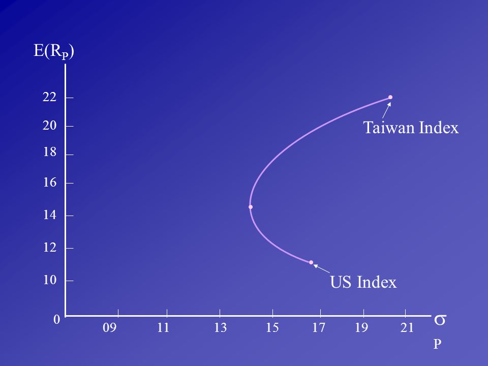
E(RP) 22 20 18 16 14 12 10 P 09 11 13 15 17 19 21
 P")
82
Efficient Portfolio E(RP) P
 P")
83
We Introduce Borrowing & Lending (p193)
2P = X12 X22 X1X2 1 2 12 (risk-free asset : 2 = 0 ) - Lending 2P = X12 12 P = X1 1 (linear combination) EP = X1R1 + X2Rf - Borrowing 2P = ( X* + 1 )2 12 + ( -X* )2 22 + 2( 1+X* )( -X* ) 12 P = (1+X*) 1 EP = (1+X*) R1 - X* Rf Portfolio Risk : Linear combination of individual risk
 - Lending. 2P = X12 12 P = X1 1 (linear combination) EP = X1R1 + X2Rf. - Borrowing. 2P = ( X* + 1 )2 12 + ( -X* )2 22 + 2( 1+X* )( -X* ) 12. P = (1+X*) 1. EP = (1+X*) R1 - X* Rf. Portfolio Risk : Linear combination of individual risk.")
84
Combination of Risky(A) and Risk Free Asset
• A Rf

85
New Efficient Portfolio
Rf A • C Old Efficient Portfolio B T D

86
• M P T is a market portfolio; M Capital Market Line CML
EP T • EM Rf M P T is a market portfolio; M Capital Market Line CML Risk-return relationship for efficient portfolios Intercept: Rf price of time slope: (EM - Rf) / M price of risk Ep = Rf + [ (EM - Rf) / M ] x P
 / M price of risk. Ep = Rf + [ (EM - Rf) / M ] x P.")
87
Systematic Risk vs. Unsystematic Risk
Capital Asset Pricing Model: CAPM Apply Portfolio Theory to evaluate all risky assets Systematic Risk vs. Unsystematic Risk We can eliminate unsystematic risk by combining securities. (it cancels each other) We can not eliminate systematic risk since it moves with market as a whole Therefore,
 We can not eliminate systematic risk since it moves. with market as a whole. Therefore,")
88
Systematic Risk = Market risk = Covariance(iM)
Required Rate of Return on Risky Asset Risk-free Rate(Rf) Risk Premium = + = Rf + amount of risk Price of risk = Rf + = Rf + = Rf +
 Risk. Premium. = + = Rf + amount of risk Price of risk. = Rf + = Rf + = Rf +")
89
STOCK BETA STOCK BETA AT&T .65 General Electric 1.29 Bristol-Myers Squibb .95 McDonald’s .95 Coca-Cola .98 Microsoft 1.26 Compaq 1.13 Reebok .87 Exxon .73 Xerox 1.25 STOCK BETA STOCK BETA BP .74 LVMH 1.00 Deutsche Bank 1.05 Nestle 1.01 Sony 1.03 Fiat 1.11 Hudson Bay Telefonia de Argentina .51 1.31 KLM 1.13

90
rf+(rm - rf) AT&T .65 10.7% Bristol-Myers Squibb .95 13.1 Coca-Cola
EXPECTED RETURN rf+(rm - rf) STOCK BETA AT&T .65 10.7% Bristol-Myers Squibb .95 13.1 Coca-Cola .98 13.3 Compaq 1.13 14.5 Exxon .73 11.3 General Electric 1.29 15.8 McDonald’s .95 13.1 Microsoft 1.26 15.6 Reebok .87 12.5 Xerox 1.25 13.9
 STOCK. BETA. AT&T % Bristol-Myers Squibb Coca-Cola Compaq Exxon General Electric McDonald’s Microsoft Reebok Xerox")
91
Summary 1) Covariance risk (normalized) iM 2M
“” 1) Covariance risk (normalized) iM 2M 2) Sensitivity of stock i’s return with respect to market Ex:
 Covariance risk (normalized) iM. 2M. 2) Sensitivity of stock i’s return with respect to. market. Ex:")
92
Security Market Line: SML
E(Ri) ? ? Rf i 1 1) CAPM Line 2) Equilibrium Line; If asset is correctly priced (in its equilibrium), in terms of CAPM, it falls on this line. Below this line : Above this line :
 Rf. i. 1. 1) CAPM Line. 2) Equilibrium Line; If asset is correctly priced (in its equilibrium), in terms of CAPM, it falls on this line. Below this line : Above this line :")
93
E(R) C • B • rm A • rf 0.5 1.0 1.5
 C • B • rm A • rf ")
94
Beta vs. Average Risk Premium
Avg Risk Premium Market line 30 20 10 10 9 8 7 6 Investors 5 3 2 1 4 Market Portfolio Portfolio Beta 1.0

95
Investors Avg Risk Premium 1931-65 Market Line 30 20 10 10 9 8 7 5 4 6
10 Investors 9 8 7 5 4 6 3 2 1 Market Portfolio Avg Risk Premium 1.0 Portfolio Beta 30 20 10 Market Line Investor 2 5 9 3 4 1 8 6 7 10 Market Portfolio Portfolio Beta 1.0

96
8.4 Some Alternative Theories
Arbitrary Pricing Theory Assumes that each stock’s return depends partly on macroeconomic factors or noise (event that are unique to company) R = a + b1rf1 + b2rf2 + b3rf3 + … … noise Expected Premium = r - rf = b1 (r1- rf ) + b2 (r2 - rf ) + b3 (r3 - rf ) + … …
 R = a + b1rf1 + b2rf2 + b3rf3 + … … noise. Expected. Premium. = r - rf = b1 (r1- rf ) + b2 (r2 - rf ) + b3 (r3 - rf ) + … …")
97
Estimated risk premium
APT example 1. Identify the Macroecnomic Factors Yield Spread Interest Rate Exchange Rate Real GNP Inflation 2. Estimate the Risk Premium for Each Factor Estimated risk premium (rfactor - rf) Factor Yield spread 5.10% Interest rate -.61 Exchange rate -.59 Real GNP .49 Inflation -.83 Market 6.63
 Factor. Yield spread. 5.10% Interest rate Exchange rate Real GNP Inflation Market")
98
3. Estimate the Factor Sensitivity
Factor risk (b) Estimated risk premium (rfactor - rf) Factor risk premium [b(rfactor - rf)] Yield spread 1.04 5.10% 5.30% Interest rate -2.25 -.61 1.37 Exchange rate .70 -.59 -.41 Real GNP .17 .49 .08 Inflation -.18 -.83 .15 Market .32 6.63 2.04 Total 8.53%
 Estimated risk. premium. (rfactor - rf) Factor risk. premium. [b(rfactor - rf)] Yield spread % 5.30% Interest rate Exchange rate Real GNP Inflation Market Total. 8.53%")
99
Capital Budgeting and Risk
Chapter 9

100
Are the New Projects More Risky or Less Risky
than its Existing Business? Each project should be evaluated at its own Cost of Capital (implication of Value Additivity Principle) Firm Value = PV(AB) = PV(A) + PV(B) = sum of separate assets PV(A), PV(B) are valued as if they were mini-firms in which stockholders invest directly.
 Firm Value = PV(AB) = PV(A) + PV(B) = sum of separate assets. PV(A), PV(B) are valued as if they were mini-firms. in which stockholders invest directly.")
101
r • B Cost of Capital • A rf

102
True Cost of Capital - depends on the use to which the capital is put - Project beta () Expected Return = r = rf + (project beta) (rm - rf) “” of project or division - Look at an average of similar companies (or industry beta) - Firm’s borrowing policy (leverage) affects its stock beta - Project beta shifts over time.
 - Firm’s borrowing policy (leverage) affects its stock. beta. - Project beta shifts over time.")
103
Industry Beta and Divisional Cost of Capital
Individual measurement error Portfolio error cancelled out If you consider across-the-board expansion, such as new division, What is the “” for new division? Answer:

104
Measuring Betas Using monthly stock return on IBM Using monthly market return (Ex) months R1IBM R1M R2IBM R2M … … … … R60IBM R60M

107
Average rate of price appreciation or depreciation,
( = alpha) Average rate of price appreciation or depreciation, born by stock-holders when investors in the market as a whole earn nothing. R-squared R2 The proportion of variance of stock price change that can be explained by market movement. means systematic risk / total risk
 Average rate of price appreciation or depreciation, born by stock-holders when investors in the market. as a whole earn nothing. R-squared R2. The proportion of variance of stock price change. that can be explained by market movement. means systematic risk / total risk.")
108
Beta = 1.30 Alpha = -.65 = -0.65% ; -0.65 12 -7.8%
Change in prices of DEC common stock Beta = 1.30 Change in market index Alpha = -.65 = -0.65% ; 12 -7.8%

109
9.2 Capital Structure & Company Cost of Capital(COC)
Cost of Capital; hurdle rate minimum return required to make firm value unchanged. Depends on also depends on * Financial leverage does not affect the risk or the expected return on the firm’s assets. But,

110
How Changing Capital Structure Affects Expected Return?
Company Cost of Capital = r Asset = r portfolio D E (WACC) = r d + r e D + E E + D (EX) B/S (market value) A 100 D 40 E 60 100 100 r d = 8% r e = 15% r Asset =
 = r d. + r e. D + E. E + D. (EX) B/S (market value) A 100. D 40. E r d = 8% r e = 15% r Asset. =")
111
(Now) : Issue 10 equity, Retire 10 debt
B/S (market value) A 100 D 30 E 70 100 100 * The change in financial structure does not affect does affect (Ex) lower leverage: rD 7.3% (Given) rAssets =
 A 100. D 30. E * The change in financial structure does not affect. does affect. (Ex) lower leverage: rD 7.3% (Given) rAssets =")
112
How does Changing Capital Structure Affect Beta?
V E V D + E Assets = Portfolio = V = D + E D = E = 1.2 A = After refinancing; D 0.1(Given)
")
113
Before Refinancing After Refinancing Expected return (%) rdebt=8
rassets=12.2 requity=15 20 .2 debt= Beta .8 assets= equity=1.2 Before Refinancing 20 Expected return (%) .1 debt= rdebt=7.3 rassets=12.2 requity=14.3 Beta .8 assets= equity=1.1 After Refinancing
 .1. debt= rdebt=7.3. rassets=12.2. requity=14.3. Beta. .8. assets= equity=1.1. After Refinancing.")
114
9.3 How to Estimate the company Cost of Capital
Pinnacle West’s Common Stock Beta Standard. Error Boston Electric . 60 . 19 Central Hudson . 30 . 18 Consolidated Edison . 65 . 20 DTE Energy . 56 . 17 Eastern Utilities Associate . 66 . 19 GPU Inc. . 65 . 18 NE Electric System . 35 . 19 OGE Energy . 39 . 15 PECO Energy . 70 . 23 Pinnacle West Corp. . 43 . 21 PP & L Resources . 37 . 21 Portfolio Average .51 .15

115
requity = rf + equity [ rm - rf]
= = 8.6% rd = 6.9%, re = 8.6%, = 0.43, = 0.57 WACC = Company Cost of Capital = rd re D V E V D V E V
![requity = rf + equity [ rm - rf]](http://slideplayer.com/slide/4257055/14/images/115/requity+%3D+rf+%2B+%EF%81%A2equity+%EF%82%B4+%5B+rm+-+rf%5D.jpg "= 0.08 = % rd = 6.9%, re = 8.6%, = 0.43, = WACC = Company Cost of Capital. = rd + re. D. V. E. V. D. V. E. V.")
116
9.4 Discount Rates for International Projects
Foreign investments are not always riskier. .47 .120 3.80 Taiwan .35 .147 2.36 Kazakhstan .62 .160 Brazil 1.46 .416 3.52 Argentina Beta coefficient Correlation Ratio s Foreign Investment in the US

117
P E(RP) Taiwan Index US Index 22 20 18 16 14 12 10 09 11 13 15 17 19
09 11 13 15 17 19 21
118
9-4 Setting Discount Rate when you can’t calculate
Avoid fudge factors Do not add fudge factors to the discount rate instead adjust cash flow forecasts (Ex) dry hole, FDA approval, politica1 unstability in foreign country etc Think about the determinant of asset beta
 dry hole, FDA approval, politica1 unstability in foreign country etc. Think about the determinant of asset beta.")
119
(Ex) Q: What are industries which are risky, but have low ?
 Q: What are industries which are risky, but have low ")
120
Determinants of Asset Beta:
Cyclicality: Firms whose revenue depend on business cycle high Operating Leverage Commitment to fixed production charges High fixed cost ratio High operating leverage High Asset Beta Why ?

121
Break Even Point Analysis
$ Total Cost Unit Variable Cost Fixed Cost Q

122
TR TC Profit Loss FC BEF Low Fixed Cost (high Variable Cost) Low OL
 Low OL")
123
TR TC FC High Fixed Cost (Low Variable Cost) High OL
 High OL")
124
9-6 Another Look at Risk and Discounted Cash flow
Risk-adjusted: t=1 PV = [Ct / (1+r)t], r = rf + (rM - rf) n (Ex) r = 8 = 12% Year CF PV 240.2 100 1.12 x = (x = certainty equivalent cash flow) x 100 = 89.3 = (1.12)2 (1.06)2 x = 100 (1.06/1.12)2 = 89.57
t], r = rf + (rM - rf) n. (Ex) r = 8 = 12% Year CF PV x = (x = certainty equivalent cash flow) x = 89.3 = (1.12)2. (1.06)2. x = 100 (1.06/1.12)2 =")
125
= 1+rf 1+r 1+rf 1+r General Solution Risky Cash Flow at time t
÷ ø ö ç è æ Risky Cash Flow at time t Certainly equivalent Cash Flow at time t = 1+rf 1+r t ÷ ø ö ç è æ We call t = Certainty equivalent coefficient 1 = (1.06 / 1.12) = 0.946 2 = (1.06 / 1.12)2 = 0.896 3 = (1.06 / 1.12)3 = 0.848 Valuing CE cash flow CE(CF) (1 + rf) CF PV = = 1 + r
 = 2 = (1.06 / 1.12)2 = 3 = (1.06 / 1.12)3 = Valuing CE cash flow. CE(CF) (1 + rf) CF. PV = = 1 + r.")
126
- (Example) E(C) = -1,000,000 0.5 = -500,000 r = 25% 125 500 +
1.25 125 (1.25)t t=2 NPV = -125 - + = or -$125,000? Convert into Certainty Equivalent cash flow: Success NPV = (250/0.1) = (50% chance) Failure NPV = 0 (50% chance) E(NPV) = 1500 0.5 = 750 (if = 0.5) NPV = = or $225,000 (750 0.5) 1.07
t. t=2. NPV = = -125 or -$125,000 Convert into Certainty Equivalent cash flow: Success. NPV = (250/0.1) = (50% chance) Failure. NPV = 0 (50% chance) E(NPV) = 1500 0.5 = 750 (if = 0.5) NPV = = or $225,000. (750 0.5)")
127
Making Sure Managers Maximize NPV
Chapter 12

128
12.1 Incentives A. Agency Problems in Capital Budgeting Reduced Effort
Perquisites Empire Building Entrenchment Avoiding Risk B. Monitoring C. Compensation

129
6 . 12 11 702 , 30 347 - Walt Disney 2 7 8 9 420 13 298 UAL 5 15 963 4 335 Safeway 1 20 885 42 3,119 Morris Philip 47 680 1,727 Microsoft 14 23.0 219 22 1,688 Merck 3 21.8 138 18 1,327 Johnson & 7.8 67,431 2,743 IBM 15.2 24,185 99 Packard Hewlett 5.9 82,887 3,527 Motors General 17.7 53,567 2,515 Electric 12.1 58,272 1,719 Motor Ford 12.2 23,024 6,81 Chemical Dow 9.7% 36.0% $10,814 $2,442 Cola Coca Capital of Cost on Return Invested EVA

130
Corporate Financing and
Market Efficiency Chapter 13

131
? B/S How to spend $? How to raise $?
So far, we assume ‘all equity’ financing. Stockholders supply all the firm’s capital, bear all the business risks, and receive all the rewards. <Questions>

132
13.1 We always come back to NPV
(ex) Government offer: $100,000, 10yrs at 3% Market fair rate: 10% NPV = Amount borrowed - PV of interest payments - PV of loan payment t=1 10 3,000 (1.10)t 100,000 (1.10)10 - = +100,000 - = $43,200 Difference between Investment & Financing Decisions Easy reverse Abandonment value is O.K. Lose or make money is not easy
 Government offer: $100,000, 10yrs at 3% Market fair rate: 10% NPV = Amount borrowed - PV of interest payments. - PV of loan payment. t= ,000. (1.10)t. 100,000. (1.10)10. - = +100,000 - = $43,200. Difference between Investment & Financing Decisions. Easy reverse Abandonment value is O.K. Lose or make money is not easy.")
133
80 130 180 Month Level 80 130 180 230 Month Level

134
13.2 Efficient Market Hypothesis
Definition Stock price reflects information immediately and completely Level of Efficiency - Weak Form Stock price reflects previous price movement immediately and completely - Semi-Strong Form all publicly available information - Strong Form all information (public, private, and insider)
")
135
Test of Market Efficiency
- Weak form - Semi-Strong form - Strong form Market Anomaly - Small firm Effect - January Effect - Weekend Effect Q: Is market inefficient?

136
The Dividend Controversy
Chapter 16

137
Q1 : How company set dividend?
Q2 : How dividend affect stock price? Investment Financing - So far: independent If dividend affects firm value, attractiveness of new project depends on where the money is coming from. Dividend Financing decision Mixed with Decision Investment Given capital budgeting & financing decision, what is the effect of change in dividend?

138
16.1 How dividends are paid? Board of directors Record date
Legal Limitation Companies are allowed to pay a dividend out of surplus but they may not distribute legal capital (par value of all outstanding shares) Share Repurchase ’80: Ford: $1.2 bil, Exxon: $15 bil, IBM, COCA etc. Just after 1987 Crash: Citi Corp $6.2 bil How to Repurchase? 1. Open market repurchase 2. Tender Offer 3. Direct negotiation
 Share Repurchase. ’80: Ford: $1.2 bil, Exxon: $15 bil, IBM, COCA etc. Just after 1987 Crash: Citi Corp $6.2 bil. How to Repurchase 1. Open market repurchase. 2. Tender Offer. 3. Direct negotiation.")
139
Greenmail Target of a takeover attempt buys off the hostile bidder by repurchasing any shares that it has acquired with premium at the expense of existing shareholders. 16.2 Information content of Dividend Signaling Model Other Signaling Tools

140
- Dividend irrelevance
16.3 Dividend Controversy MM(1961) - Dividend irrelevance In a world without taxes and transaction costs (efficient and perfect capital market) (Ex) B/S (Market Value) Cash 1,000 D FA ,000 10,000+NPV E 10,000 + NPV 10,000 + NPV Pay dividend by issuing new shares($1,000) We want to continue project w/t cash($1,000)
 - Dividend irrelevance. In a world without taxes and transaction costs. (efficient and perfect capital market) (Ex) B/S (Market Value) Cash 1, D. FA 9, ,000+NPV E. 10,000 + NPV. 10,000 + NPV. Pay dividend by issuing new shares($1,000) We want to continue project w/t cash($1,000)")
141
Value of original shareholders’ shares (Ex Post)
= Value of company - Value of new shares = (10,000 + NPV) - 1,000 = $ 9,000 + NPV $1,000 cash dividend = $1,000 capital loss Investment and borrowing policies are unaffected by dividend [overall value 10,000 + NPV, is unchanged] * Crucial Assumption New stock holders pay fair-price Old stockholders have received $1,000 dividend and $1,000 capital loss Dividend policy doesn’t matter.
 - 1,000 = $ 9,000 + NPV. $1,000 cash dividend = $1,000 capital loss. Investment and borrowing policies are unaffected by dividend. [overall value 10,000 + NPV, is unchanged] * Crucial Assumption. New stock holders pay fair-price. Old stockholders have received $1,000 dividend. and $1,000 capital loss. Dividend policy doesn’t matter.")
142
(Ex) N = 1,000 shares NPV = $2,000 Vold = Vold* = Number of new shares sold =
 N = 1,000 shares NPV = $2,000 Vold = Vold* = Number of new shares sold =")
143
The Rightist Trade a safe receipt with an uncertain future gain? Sell it! Market Imperfection Transaction costs Temporarily depressed price Information asymmetry about future Earning The Leftist Tax Argument Weakened after 1986 ‘Tax Reform Act’

144
16.6 Middle of the Roaders Without tax and transaction cost (perfect & efficient market), company’s value is not affected by dividend policy (irrelevant): MM (1961) Even if with tax and other imperfections, Q: If company increase stock price by paying more or less dividend, why have not they already done so? (perhaps) “Supply Effect”
, company’s value is not affected by dividend policy (irrelevant): MM (1961) Even if with tax and other imperfections, Q: If company increase stock price by paying more or less dividend, why have not they already done so (perhaps) Supply Effect")
145
Does Debt Policy Matter?
Chapter 17

146
MM Proposition I B/S Asset Structure Capital Structure
Mix of different securities “Maximize V” MM Proposition I Firm can not change the total value of securities just by splitting its cash flows into different streams. (RHS) Firm value is determined by its real assets. (LHS)
 Firm value is determined by its real assets. (LHS)")
147
17.1 The Effect of Leverage in a Tax Free Economy
VU: Value of unlevered firm EL = VL - DL 1) 1% of unlevered firm $ investment $ return (NOI) .01 VU profit
 1% of unlevered firm. $ investment $ return (NOI) .01 VU .01 profit.")
148
2) 1% of equity & debt of levered firm (I: interest)
$ invest $ return Debt .01 DL .01 I NI .01 EL .01(DL + EL) .01 (profit -I) .01 profit Equity = .01 VL same profit (NOI) same cost (same investment) VU = VL
 .01 (profit -I) .01 profit. Equity. = .01 VL. same profit (NOI) same cost (same investment) VU = VL.")
149
same cost (same investment)
3) Buy 1% of equity of levered firm $ investment $ return .01 EL (profit -I) = .01 (VL - DL) 4) Alternative way: Borrow .01 DL on your account Buy 1% of equity of unlevered firm $ investment $ return Borrowing Equity -.01 DL -.01 I .01 VU .01 profit .01(VU - DL) .01 (profit - I) Same profit VU = VL same cost (same investment)
 Buy 1% of equity of levered firm. $ investment $ return. .01 EL .01 (profit -I) = .01 (VL - DL) 4) Alternative way: Borrow .01 DL on your account. Buy 1% of equity of unlevered firm. $ investment $ return. Borrowing. Equity DL I. .01 VU. .01 profit. .01(VU - DL) .01 (profit - I) Same profit. VU = VL. same cost (same investment)")
150
All Equity Example of Proposition I (p.477) P = $10 VU = $10,000
E(EPS) = $1.5, P = $10, E(R) = 1.5/10 = 15% N = 1,000 P = $10 VU = $10,000 NOI($) , , ,000 EPS($) ROE(%) A
 = $1.5, P = $10, E(R) = 1.5/10 = 15% N = 1,000. P = $10. VU = $10,000. NOI($) 500 1,000 1,500 2,000. EPS($) ROE(%) A.")
151
debt $5000, k = 10%, repurchase: 500 shares
Issue: debt $5000, k = 10%, repurchase: 500 shares N = 500 P = $10, k = 10% Market value of stock: $5,000 Market value of debt : $5,000 NOI($) , , ,000 Interest NI($) , ,500 EPS($) 1 2 3 ROE(%)
 500 1,000 1,500 2,000. Interest NI($) ,000 1,500. EPS($) ROE(%)")
152
3.00 Equal proportions debt and equity 2.50 Expected EPS with debt and equity 2.00 All equity Expected EPS with all equity 1.50 1.00 .50 Expected operating income 500 1000 1500 2000

153
Personal Leverage NOI($)
C Borrow $10, then invest $20 in two unlevered shares (Initially, I have $10) NOI($) 500 1,000 1,500 2,000 Earnings on two shares($) 1 2 3 4 Interest($) at 10% -1 -1 -1 -1 Net Earnings($) 1 2 3 Return on 0% 10% 20% 30% $10 investment
 NOI($) ,000. 1,500. 2,000. Earnings on two shares($) Interest($) at 10% Net Earnings($) Return on. 0% 10% 20% 30% $10 investment.")
154
17.2 How Leverage Affects Return
Current structure all equity Proposed structure E(EPS) $1.5 $2.0 NOI = $1,500 V=10,000 P $10 $10 N =1,000 D=5,000 E(ROE) 15% 20% Kd = 10% E=5,000 Leverage increases EPS, but not P. The change in EPS is exactly offset by a change in the rate at which the earning are capitalized. 15% 20%
 $1.5. $2.0. NOI = $1,500. V=10,000. P. $10. $10. N =1,000. D=5,000. E(ROE) 15% 20% Kd = 10% E=5,000. Leverage increases EPS, but not P. The change in EPS is exactly offset by a change in the. rate at which the earning are capitalized. 15% 20%")
155
Expected return on asset(rA) NOI = Market value of all security Assumption: In a perfect market, borrowing decision does not affect operating income or total market value of its securities. Borrowing decision does not affect expected return on firm’s assets(rA).
.")
156
rA rE rD rE rA D D+E E = + D+E = + D E (rA - rD) - Expected
return on debt Expected return on equity Expected return on assets Debt/ Equity Ratio Expected return on assets + - =

157
Proposition II (MM) The expected return on equity (rE) of a levered firm increases in proportion to debt to equity ratio (D/E) & the rate depends on the spread between rA and rD. (Ex) rA = 15% D = 5,000 rD = 10% E = 5,000 rE =
 of a levered firm increases in proportion to debt to equity ratio (D/E) & the rate depends on the spread between rA and rD. (Ex) rA = 15% D = 5,000. rD = 10% E = 5,000. rE =")
158
rE rA rD rD r = = = Figure 17-2 Expected Return on Equity
MM’s proposition II. The expected return on equity rE increases linearly with the debt-equity ratio so long as debt is risk-free. But if leverage increases the risk of the debt, debtholders demand a higher return on the debt. This causes the rate of increase in rE to slow down. rE Expected Return on Equity = rA Expected Return on Assets = rD rD Expected Return on Debt = D E Risk free debt Risky debt

159
The Risk-Return Trade-off
= D + E E E A + D E (A D) - = Investors (stock-holders) require higher returns on levered equity
 - = Investors (stock-holders) require higher returns. on levered equity.")
160
17.3 The Traditional Position
Moderate degree of financial leverage may increase rE although not to the degree predicted by MM proposition II Excessive debt raise rE faster rA (=WACC) decline & later rise.
 decline & later rise.")
161
r rE rE rA rA rD rD = = = = (MM) (traditional) (MM) (traditional) D E
debt equity = Traditionalist believe there is an optimal debt-equity ratio that minimizes rA

162
B Transaction Costs Imperfections may allow firms that borrow to provide valuable service. (Ex. Economies of scale in borrowing) Levered Shares might trade at premium compared to their theoretical value in perfect market Smart financial engineer already recognize this and shift capital structure to satisfy this client.

163
How Much Should a Firm Borrow?
Chapter 18

164
Question: Why do we worry about debt policy?
Evidence: 1. D/E ratio are different across the industry. 2. Imperfections: Tax Bankruptcy Costs (T.C.) Cost associated with financial distress Potential conflicts of interests between security holders Interactions of investment and financing decision
 Cost associated with financial distress. Potential conflicts of interests between security holders. Interactions of investment and financing decision.")
165
18.1 Corporate Taxes Income statement of Firm U of Firm L Earnings before interest and taxes Interest paid to bondholders Pretax income Tax at 35% Net income to stockholders Total income to both bondholders and stockholders Interest tax shield (.35interest) $1,000 80 1,000 920 350 322 $650 $598 $ = $650 $ = $678 28
 $1, , $650. $598. $ = $650. $ = $")
166
rD (rD rD Interest Payment = D TC D) PV(Tax shield) = = TC D
• rD PV(Tax shield) = = TC D 0.35 0.08 1000 PV(Tax shield) = 0.08 = $350
 = = TC. D 0.08 PV(Tax shield) = = $350.")
167
Normal Balance Sheet(Market Values)
Asset value (present value of after-tax cash flows) Debt Equity Total assets Total value Expanded Balance Sheet(Market Values) Pretax asset value (present value of pretax cash flows) Debt Government ‘s claim (present value of future taxes) Equity Total pretax assets Total value
 Debt. Equity. Total assets. Total value. Expanded Balance Sheet(Market Values) Pretax asset value (present. value of pretax cash flows) Debt. Government ‘s claim. (present value of future. taxes) Equity. Total pretax assets. Total value.")
168
Book Values Market Values Net working capital Long-term debt
Table 18.3(a) Book Values Net working capital Long-term debt $2,644 $1,347 Other long-term liabilities Long-term assets 17,599 6,282 12,614 Equity Total assets $20,243 $20,243 Market Values Net working capital $2,644 $1,347 Long-term debt Market value of long-term assets Other long-term liabilities 131,512 6,282 126,527 Equity Total assets $134,156 $134,156 Total value
 Book Values. Net working capital. Long-term debt. $2,644. $1,347. Other long-term. liabilities. Long-term assets. 17,599. 6, ,614. Equity. Total assets. $20,243. $20,243. Market Values. Net working capital. $2,644. $1,347. Long-term debt. Market value of. long-term assets. Other long-term. liabilities. 131,512. 6, ,527. Equity. Total assets. $134,156. $134,156. Total value.")
169
Book Values Market Values Net working capital Long-term debt
Table 18.3(b) Book Values Net working capital Long-term debt $2,644 Other long-term liabilities 6,282 Long-term assets 17,599 11,614 Equity Total assets $20,243 $20,243 Market Values Net working capital $2,644 Long-term debt Market value of long-term assets Other long-term liabilities 131,512 6,282 Additional tax shields Equity Total assets Total value
 Book Values. Net working capital. Long-term debt. $2,644. Other long-term. liabilities. 6,282. Long-term assets. 17, ,614. Equity. Total assets. $20,243. $20,243. Market Values. Net working capital. $2,644. Long-term debt. Market value of. long-term assets. Other long-term. liabilities. 131,512. 6,282. Additional tax shields. Equity. Total assets. Total value.")
170
MM & Taxes: MM Prop I with corporate tax.
VL = VU + PV (Tax Shield) 100% debt?
 100% debt")
171
18.2 Corporate and Personal Taxes
Operating income $1.00 Corporate tax Income after corporate tax Personal tax Income after all taxes

172
Corporate Borrowing is better
If (1 - TP) > (1- TPE) * (1 - Tc) Relative Tax Advantage of Debt = Special Cases: 1. TPE = TP, RTAD = MM’s original 2. (1 - TP) = (1 - TPE) * (1 - Tc) RTAD = 1.0 Debt policy is irrelevant! This case happen when Tc < TP & TPE is small. (1 - TP) (1 - TPE) • (1 - Tc) 1 (1 - TC)
 > (1- TPE) * (1 - Tc) Relative Tax Advantage of Debt = Special Cases: 1. TPE = TP, RTAD = MM’s original. 2. (1 - TP) = (1 - TPE) * (1 - Tc) RTAD = 1.0. Debt policy is irrelevant! This case happen when Tc < TP & TPE is small. (1 - TP) (1 - TPE) • (1 - Tc) 1. (1 - TC)")
173
(Ex) Tc = 35%, TP = 39.6% What TPE makes debt policy irrelevant?
 Tc = 35%, TP = 39.6% What TPE makes debt policy irrelevant")
174
18.3 Cost of Financial Distress
Value of firm (levered) Value of all equity + PV(tax shield) = - PV (costs of financial distress) Market Value of The Firm Debt
 Value of all. equity. + PV(tax shield) = - PV (costs of financial distress) Market Value of The Firm. Debt.")
175
(unlimited liability)
Bankruptcy Costs ACE LIMITED (limited liability) ACE LIMITED (unlimited liability) Payoff to bondholders Payoff to bondholders Payoff Payoff 1,000 1,000 500 500 Asset value Asset value 500 1,000 500 1,000 Payoff to stockholders Payoff to stockholders Payoff Payoff 1,000 1,000 Asset value Asset value 500 1,000 500 1,000 -1,000 -1,000
 ACE LIMITED. (unlimited liability) Payoff to. bondholders. Payoff to. bondholders. Payoff. Payoff. 1,000. 1, Asset. value. Asset. value , ,000. Payoff to. stockholders. Payoff to. stockholders. Payoff. Payoff. 1,000. 1,000. Asset. value. Asset. value , , , ,000.")
176
Direct: legal fee, court fee, etc. Indirect: difficult to measure
Table 18.4 SHARE PRICE FRIDAY APR 10, 1987 MONDAY APR 13, 1987 CHANGE NUMBER OF SHARES (MILLIONS) IN VALUE Texaco Pennzoil Total $31.875 $28.50 -$3.375 242 -$ 817 -628 92.125 77.00 41.5 -$1,445
 IN VALUE. Texaco. Pennzoil. Total. $ $ $ $ $1,445.")
177
Financial Distress without Bankruptcy
When firms get into trouble, stockholders’ & bondholders’ interests conflict. reduce value of firm Circular File company (Book Values) Net working capital $ 20 Fixed assets 80 Total assets $100 $ 50 50 Bonds outstanding Common stock Total value Circular File company (Market Values) Net working capital $20 Fixed assets 10 Total assets $30 $25 5 Bonds outstanding Common stock Total value
 Net working capital. $ 20. Fixed assets. 80. Total assets. $100. $ Bonds outstanding. Common stock. Total value. Circular File company (Market Values) Net working capital. $20. Fixed assets. 10. Total assets. $30. $ Bonds outstanding. Common stock. Total value.")
178
Risk Shift: The First Game
(Ex1) C0 C1 $120 (p=10%) -$10 $ 0 (p=90%) If r=50%, NPV = -10 + 1200.1+0 1.5 = -$2 Circular File company (Market Values) Net working capital $10 Fixed assets 18 Total assets $28 $20 8 Bonds outstanding Common stock Total value
 C0. C1. $120. (p=10%) -$10. $ 0. (p=90%) If r=50%, NPV = = -$2. Circular File company (Market Values) Net working capital. $10. Fixed assets. 18. Total assets. $28. $ Bonds outstanding. Common stock. Total value.")
179
(Ex2): Amount of Debt = $600 High Risk Project Good (p=0.5) Bad (p=0.5) V 2,000 300 D S V = D = S =

180
Low Risk Project Good (p=0.5) Bad (p=0.5) V 1,400 1,000 D S V = D = S =
 Bad (p=0.5) V 1,400 1,000 D S V = D = S =")
181
Refusing to contribute equity capital: The second game
Good project with NPV= + $5 by investing $10 Net working capital $20 $33 Bonds Fixed assets 25 12 Common stock Total assets $45 $45 Total value Firm value increase by $15 Bond value increase by $8 Stock value increase by $7

182
Cost of Distress Vary with Type of Asset
Firms with intangibles having value only as a part of going concern, high technology, investment opportunities, human capital, lose more in the financial distress.

183
Trade off Theory of Capital Structure
Trade-off between interest tax shield and the costs of financial distress Company with safe, tangible asset and plenty of taxable income High debt ratio Unprofitable company with risky, intangible assets Equity finance Trade-off theory explains what kinds of companies “go private in LBO” Trade-off theory cannot explain why some most successful companies thrive with little debt.

184
18.4 The Pecking Order of Financing Choice, Information Asymmetry
Asymmetric information affects the choice between internal and external financing and between new issues of debt and equity securities Pecking order: internal fund, new issue of debt, finally new issue of equity (Exception) Firm with already excessive debt High-tech, high-growth company
 Firm with already excessive debt. High-tech, high-growth company.")
185
Implication of Pecking Order
1. Firms prefer internal financing 2. Firms adopt target payout ratio & try to avoid sudden changes in dividend 3. Sticky dividend policy 4. If external finance is required, debt, convertible bond, then equity Financial Slack: Cash, marketable securities, readily saleable real assets, & ready access to the debt market or to bank financing More valuable to firm with plenty of positive-NPV growth opportunity

186
Interactions of Investment and Financing Decisions
Chapter 19

187
Introduction So far, all equity financing
All financing decisions are irrelevant In this chapter,we consider capital budgeting decision when investment and financing decision interact and can not be separated

188
NPV of financing decisions caused by project acceptance Base NPV APV = + (value additivity principle)
 .")
189
rD rE rD (1-Tc) rE 19.1 After-tax WACC D E WACC = + V V D E WACC = + V
 rE 19.1 After-tax WACC D E WACC = + V V D E WACC = + V")
190
Sangria Corporation (Book Values, millions) (Market Values, millions)
Asset $100 $50 Debt 50 Equity Total assets $100 $100 Total value (Market Values, millions) Asset $125 $50 Debt 75 Equity Total assets $125 $125 Total value
 Asset. $125. $50. Debt. 75. Equity. Total assets. $125. $125. Total value.")
191
WACC =? rD rE =0.08 =0.146 TC =0.35 D V E V = = WACC =

192
Invest: $12.5 million $ 7.5 million (Equity) $ million (Debt) Pretax cashflow: $2.085 (perpetual) Tax: 35% After-tax cashflow: $1.355 million NPV = Return on Investment =

193
Return on Equity: NOI 2.085 -0.4 (=0.085) I Earning After tax 1.685 -Tax -0.59 (=1.6850.35) 1.095 1.095 Expected return on Equity = = 0.146 7.5 E(RE) = rE NPV=0
 = rE. NPV=0.")
194
19.2 Using WACC - Some tricks of the trade
Current Assets, Current liabilities, including cash, inventory, including accounts payable and accounts receivable and short-term debt Plant and equipment Long-term debt (D) Preferred stock (P) Growth opportunities Equity (E) Firm value (V) Total capitalization (V)
 Preferred stock (P) Growth opportunities Equity (E) Firm value (V) Total capitalization (V)")
195
Industry Cost of Capital
Cost of capital of new subsidiary Company’s WACC vs. a weighted-average cost of capital of for a portfolio of industry An Application of the Railroad Industry Aggregate industry capital structure in 1979 Debt Equity $24,383 bil $57,651 bil 29.7% 70.3% rd=7.2%, g=11.5%, D/P= 2.3%, TC = 35% rE = WACC =

196
Valuing Companies: WACC vs. Flow-to-Equity Method WACC
Debt ratio is expected to be constant Calculate tax as if firm is all equity-financed Usually forecast to a median-time horizon and add a terminal value to the cashflow in the horizon year Discount at WACC evaluation of the assets and operation of the firm

197
rE=rA + (rA-rD)(1-TC) Flow-to Equity Method Evaluation of equity
Discount the cashflow to equity, after interest and taxes, at the cost of equity Leverage change cost of equity change two methods give different answer D E rE=rA (rA-rD)(1-TC)
(1-TC)")
198
r 19.3 Adjusting WACC when debt ratios or business risks change
Cost of Equity(rE) Rate of return Opportunity cost of capital (r) r WACC Cost of Debt(rD) Debt-Equity Ratio
 Rate of. return. Opportunity cost of capital (r) r. WACC. Cost of Debt(rD) Debt-Equity Ratio.")
199
rD rE r rE rA (Ex) D V D V = 0.4 = 0.2 (rA- rD)
Step1: unlevering the WACC Calculate opportunity cost of capital rD D V rE E + r = * If taxes are left out, WACC equals the r and is independent of leverage Step2: Estimate rD at 20% debt ratio, & Calculate new rE rE rA (rA- rD) D E + = Step3: Recalculate the WACC at the new financing weight
 D. E. + = Step3: Recalculate the WACC at the new financing. weight.")
200
r = rE= Step1: current = 0.4 Step2: rd = 8%, when = 0.2 Step3: WACC= D
V Step1: current = 0.4 r = D V Step2: rd = 8%, when = 0.2 rE= Step3: WACC=

201
Opportunity cost of capital (r)
Rate of return, percent 14.6 Cost of Equity(rE) 14 13.0 Opportunity cost of capital (r) 12 11.4 10.84 WACC 10 Cost of Debt(rD) 8.0 8 Debt-Equity Ratio(D/E) .25 .67 (D/V = .2) (D/V = .4)
 Opportunity cost of capital (r) WACC. 10. Cost of Debt(rD) Debt-Equity Ratio(D/E) (D/V = .2) (D/V = .4)")
202
Unlevering and Relevering
asset = debt ( ) + equity( ) - Relevering D E equity = asset + (asset - debt) D E or ( ) asset , if debt = “0” *. Underlying assumption: Rebalancing Maintain the same market-value debt ratio
 + equity( ) - Relevering D. E. equity = asset + (asset - debt) D. E. or (1+ ) asset. , if debt = 0 *. Underlying assumption: Rebalancing. Maintain the same market-value debt ratio.")
203
19.4 The Adjusted Present Value Rule
Base-NPV NPV = [1.8 / (1.12)t ] = $0.17 mil Issue costs. 5% of gross proceeds of issue APV = base NPV - issue cost = .17 mil - 526,000 = -356,000 Reject it! Additions to the Firm’s debt capacity APV = base NPV + PV tax-shield t=1 10
t ] = $0.17 mil. Issue costs. 5% of gross proceeds of issue. APV = base NPV - issue cost. = .17 mil - 526,000 = -356,000 Reject it! Additions to the Firm’s debt capacity. APV = base NPV + PV tax-shield. t=")
204
Table 19-1 Calculating the present value of interest tax shields on debt supported by the solar heater project (dollar figures in thousands) Debt Outstanding Interest Present Value Year at Start of Year Interest Tax Shield of Tax Shield 1 $ 5,000 $400 $140 $129.6 2 4,500 360 126 108.0 3 4,000 320 112 88.9 4 3,500 280 98 72.0 5 3,000 240 84 57.2 6 2,500 200 70 44.1 7 2,000 160 56 32.6 8 1,500 120 42 22.7 9 1,000 80 28 14.0 10 500 40 14 6.5 Total: $576 Assumptions: 1. Marginal tax rate = Tc = .35; tax shield = .35 x interest. 2. Debt principal repaid at end of year in ten $500,000 installments. 3. Interest rate on debt is 8 percent. 4. Present value calculated at the 8 percent borrowing rate. The assumption here is that the tax shields are just as risky as the interest payments generating them.

205
APV = 170, ,000 = $746,000 The value of interest Tax Shield (ITS). We treat the interest tax shield as safe cash-inflow & discount at 8%. We assume firm can capture interest tax shields of 35cents on every dollar of interest. You can’t use interest tax shield unless you pay taxes. Corporate tax favors debt. Personal tax favors equity. A project’s debt capacity depends on how well it does.

206
APV for the Perpetual Crusher project
Base case NPV = /0.12 = $1.29 mil Financing Rule 1: Debt fixed Financing Rule 2: Debt rebalanced Under rule 1 PV (tax shield) = [0.350.08 5] ÷ 0.08 = $1.75 mil APV = = $3.04 mil Under rule 2 Debt is rebalanced to 40% of actual project value. debt levels are not known & depend on the project’s actual performance. cost if capital is 12% PV(tax shield) = (0.35 0.08 5) 0.12 = $1.17 mil APV = = $2.36 mil
 = [0.350.08 5] ÷ 0.08 = $1.75 mil. APV = = $3.04 mil. Under rule 2. Debt is rebalanced to 40% of actual project value. debt levels are not known & depend on the. project’s actual performance. cost if capital is 12% PV(tax shield) = (0.35 0.08 5) 0.12 = $1.17 mil. APV = = $2.36 mil.")
207
A. Technical Point on Financing Rule 2
Discount at opportunity cost of capital Multiply the resulting PV by (1+r) and divide by (1+rD) 0.14 0.12 PV(approx) = = 1.17 1.12 1.08 PV(exact) = 1.17 = 1.21 APV = = $2.5 mil
 and. divide by (1+rD) PV(approx) = = PV(exact) = = APV = = $2.5 mil.")
208
APV and hurdle Rates APV tells whether a project makes a net contribution to the value of the firm It tells break-even cashflow CF r Tax Shield APV = - Investment + PV CF 0.12 Tax Shield (Ex) APV = - 10 + PV CF 0.12 APV = - 10 = 0 CF = 1.084 IRR = 10.84%
 APV = PV. CF APV = = 0. CF = IRR = 10.84%")
209
Adjusted Cost of Capital
General Definition of Adjusted Cost of Capital The Opportunity Cost of Capital (r) The expected rate of return offered in capital markets by equivalent-risk assets. This depends on the risk of the project’s cash flows. The Adjusted Cost of Capital (r*) Adjusted opportunity cost or hurdle rate that reflects the financing side effects of an investment project
 The expected rate of return offered in capital markets. by equivalent-risk assets. This depends on the risk of the project’s cash flows. The Adjusted Cost of Capital (r*) Adjusted opportunity cost or hurdle rate that reflects. the financing side effects of an investment project.")
210
Spotting and Valuing Options
Chapter 20

211
20.1 Call vs. Put Call: Right to buy underlying asset at a specified price Put: Right to sell underlying asset at a specified price American: Exercise anytime European: Exercise only at an expiration date Exercise Date Exercise Price Price of Call Options Put Options October 1998 January 1999 $80 80 85 $8.875 11.375 8.625 $3.25 4.75 6.875

212
(b) (a) (c) Value of Call Value of Put 85 85 85 Share Price Share
of Share 85 Share Price 85 (c)
")
213
Selling Calls, Puts, and Shares
85 85 Share Price Share Price -85 -85 Value of Call Seller’s Position Value of Put Seller’s Position (a) (a) 85 Share Price -85 Value of Stock Seller’s Position (c)
 (a) 85. Share. Price Value of Stock Seller’s Position. (c)")
214
+ = $85 $85 $85 Value of Share Your Payoff Your Payoff Buy Share
Sell call + = Future Stock Price $85 Future Stock Price $85 $85 Future Stock Price

215
+ = $85 $85 $85 Value of Share Your Payoff Your Payoff Buy Share
Buy Put + = $85 Future Stock Price $85 Future Stock Price $85 Future Stock Price

216
+ = $85 $85 $85 $85 Value of Share Your Payoff Your Payoff Buy Call
Bank deposit paying $85 $85 + = $85 Future Stock Price $85 Future Stock Price $85 Future Stock Price

217
Put - Call Parity C + PV (Ex) = P + S Expiration Date S* EX
Today S* EX S* < EX V1=C+PV(EX) V2=P+S
 V2=P+S.")
218
The Difference between Safe & Risky Bonds
Bond holder: Effectively acquire a firm Stock holder: Effectively purchase a call option on the assets of firm (PB=promised payment to bondholders) Circular File Co. (MV) Asset value $30 $25 Bond: Asset - Call 5 Stock: Call $30 $30 Firm: Asset
 Circular File Co. (MV) Asset value. $30. $25. Bond: Asset - Call. 5. Stock: Call. $30. $30. Firm: Asset.")
219
Stockholders’ Position V<50 S = V50 S =
V Ex= $50 (Promised Payment to Bondholders)
")
220
Bondholders’ Position V<50 B = V50 B =
V Ex= $50 (Promised Payment to Bondholders)
")
221
PB: Promised Payment to Bondholders (safe)
V : Firm value (asset) S : Stock value B : Risky bond value C+ PV(EX) = P + S ? S+ PV(PB) = P + V S+ B = V B = V - S = PV(PB) - P Value of riskless debt Value of risky debt = - “p”
 S : Stock value. B : Risky bond value. C+ PV(EX) = P + S. S+ PV(PB) = P + V. S+ B = V. B = V - S = PV(PB) - P. Value of. riskless. debt. Value of. risky debt. = - p")
222
Circular File Co. (Market Value)
Asset value $30 $25 Bond value = present value of promised payment - value of put 5 Stock value = asset value - present value of promised payment + value of put $30 $30

223
(Ex) Incentive program:
Spotting the Option (Ex) Incentive program: Paid bonus of $50,000 for every $ that price of stock exceeds $120. Maximum bonus is set at $2 million Pay off 120 Stock Price $40 160
 Incentive program: Paid bonus of $50,000 for every $ that. price of stock exceeds $120. Maximum. bonus is set at $2 million. Pay off Stock Price. $")
224
Buy call with exercise price of $120 and
Pay off 120 160 Stock Price Buy call with exercise price of $120 and Sell call with exercise price of $160 * Any set of contingent payoffs can be valued as a mixture of simple options on that assets

225
20.3 What determines option values?
of call Upper bound: Value of call equals share price B Lower bound: Value of call equals payoff if exercised immediately C A Share Price Exercise price

226
Payoff to call option on firm X’s shares Probability distribution of future price of firm X’s shares Payoff to option on X Payoff to call option on firm Y’s shares Exercise price Probability distribution of future price of firm Y’s shares Payoff to option on Y Exercise price

227
Y X Upper bound Lower bound Share Price Exercise price Value of calls
on shares of firms X and Y Upper bound Y Lower bound X Share Price Exercise price

228
What the price of a call options depends on
1. Increase in variables: If there is an increase in: The changes in the call option price are: Stock price (P) Exercise price(EX) Interest rate (rf) Time to expiration(t) Volatility of stock price () Positive Negative 2. Other properties: a. Upper bound. The option price is less than the stock price b. Lower bound. The option price never falls below the payoff to immediate exercise (P-EX or zero, whichever is larger) c. If the stock is worthless, the option is worthless d. As the stock price becomes very large, the option price approaches the stock price less the present value of the exercise price
 Exercise price(EX) Interest rate (rf) Time to expiration(t) Volatility of stock price () Positive. Negative. 2. Other properties: a. Upper bound. The option price is less than the stock price. b. Lower bound. The option price never falls below the payoff. to immediate exercise (P-EX or zero, whichever is larger) c. If the stock is worthless, the option is worthless. d. As the stock price becomes very large, the option price approaches. the stock price less the present value of the exercise price.")
229
rf =2.5% 20.4 An Option-Valuation Model
Constructing Option Equivalents from common stocks & borrowing Stock Price Today Stock Price 6 months later Call $68 $85 $106.25 rf =2.5% Exercise price = $85

230
Hedge ratio (Option delta):
Number of shares that are needed to replicate on call Option delta Spread of option prices = Spread of share prices = How much to borrow? Present value of the different between the payoff from the option and the payoff from the option delta number of shares PV(37.78) = $36.86 Amount of borrowing
 = $ Amount of borrowing.")
231
Buy shares and borrow $36.86 today
Option Equivalents: 5 9 Buy shares and borrow $36.86 today 6 month later Today S* = $68 S* = $106.25 5 9 Buy shares Borrow $36.36 Value of call today = value of shares - $36.86 bank loan =

232
Arbitrage Opportunity
EX 1: If call is priced at $12 : overpriced Strategy: Sell a call option Buy 5/9 share & borrow today 6 month later Today S* = $68 S* = $106.25 +12 -47.22 +36.86 + $ 1.64

233
EX 2: If call is priced at $9 : underpriced
Strategy: Buy a call option Sell 5/9 share of stock short & lend(deposit) $36.86 today 6 month later Today S* = $68 S* = $106.25 - 9 +47.22 -36.86 + $ 1.36
 $36.86 today. 6 month later. Today. S* = $68. S* = $ $")
234
Pu = probability of stock price increase in the hypothetical
Risk-Neutral Valuation: All investors are indifferent about risk Expected Return on any risky assets = rf = E(R) = Pu Ru + Pd Rd 85 Ru = = 68-85 85 Rd = = E(R) = Pu ( ) + Pd ( ) = where, Pu + Pd = 1 Pu = probability of stock price increase in the hypothetical risk-neutral world Pu = Pd = at t=1 E(C1) = at t=0 C0 =
 = Pu Ru + Pd Rd Ru = = Rd = = E(R) = Pu ( ) + Pd ( ) = where, Pu + Pd = 1. Pu = probability of stock price. increase in the hypothetical. risk-neutral world. Pu = Pd = at t=1. E(C1) = at t=0. C0 =")
235
Valuing the Intel Put Option
S P EX=$85 $68 $85 $106.25 Option delta Spread of option prices = Spread of share prices = = shares Intel share & Lend $ How is it computed?

236
Value of put = - of share + $46.07 bank loan
6 month later Today S* = $68 S* = $106.25 4 9 Sell shares Lend $46.07 4 9 Value of put = of share + $ bank loan =

237
20.5 The Black -Scholes Formula
Construct a situation where the stock price is changing continuously and generate a continuum of possible six month prices Replicate a call option by a levered investment in the stock by adjusting the degree of leverage continuously Value of call = (delta Share price) - (bank loan) [N(d1) P] [N(d2) PV(EX)]
 - (bank loan) [N(d1) P] [N(d2) PV(EX)]")
238
Value of call=[N(d1) P] + [N(d2) PV(EX)]
where Log[P/PV(EX)] t d1 + = t 2 d2 = d1 - t N(d) = cumulative normal probability density function EX = exercise price of option; PV(EX) is calculated by discounting at the risk-free interest rate, rf t = number of periods to exercise date P = price of stock now = standard deviation per period of (continuously compounded) rate of return on stock
![Value of call=[N(d1) P] + [N(d2) PV(EX)]](http://slideplayer.com/slide/4257055/14/images/238/Value+of+call%3D%5BN%28d1%29+%EF%82%B4+P%5D+%2B+%5BN%28d2%29+%EF%82%B4+PV%28EX%29%5D.jpg "where. Log[P/PV(EX)] t. d1. + = t. 2. d2. = d1. - t. N(d) = cumulative normal probability density function. EX = exercise price of option; PV(EX) is calculated. by discounting at the risk-free interest rate, rf. t = number of periods to exercise date. P = price of stock now. = standard deviation per period of. (continuously compounded) rate of return on stock.")
239
Real Options Chapter 21

240
Real Option Option to make follow-on investment if the immediate investment project succeeds. Option to abandon a project Option to wait before investing Option to vary the firm’s output or its production methods

241
21.1 The value of follow-on investment
Table 21-1 Summary of cash flows and financial analysis of the Mark I microcomputer (millions of dollars) Year 1982 1983 1984 1985 1986 1987 After-tax operating -200 +110 +159 +295 +185 cash flow (1) * Capital Investment (2) 250 Increase in working 50 100 100 -125 -125 capital (3) Net Cash Flow -450 +60 +59 +195 +310 +125 (1) - (2) - (3) NPV at 20% = - $46.45, or about -$46 million
 Year After-tax operating cash flow (1) * Capital Investment (2) 250. Increase in working capital (3) Net Cash Flow (1) - (2) - (3) NPV at 20% = - $46.45, or about -$46 million.")
242
Table 21-2. Valuing the option to invest in the Mark II microcomputer.
Assumptions 1. The decision to invest in the Mark II must be made after 3 years, in 1985. 2. The Mark II investment is double the scale of the Mark I (note the expected rapid growth of the industry). Investment required is $900 million (the exercise price), which is taken as fixed. 3. Forecasted cash inflows of the MarkII are also double those of the MarkI, which present value of about $800 million in 1985 and 800/(1.2)3 = $463 million in 1982. 4. The future value of the Mark II cash flows is highly uncertain. This value evolves as a stock price does with a standard deviation of 35 percent per year.(Many high-technology stocks have standard deviation higher than 35%.) 5. The annual interest rate is 10 percent.
. Investment. required is $900 million (the exercise price), which is taken. as fixed. 3. Forecasted cash inflows of the MarkII are also double those. of the MarkI, which present value of about $800 million in and 800/(1.2)3 = $463 million in The future value of the Mark II cash flows is highly uncertain. This value evolves as a stock price does with a standard deviation. of 35 percent per year.(Many high-technology stocks have. standard deviation higher than 35%.) 5. The annual interest rate is 10 percent.")
243
Interpretation The opportunity to invest in the Mark II is a 3-year call option on asset worth $463 million with a $900 million exercise price. Valuation 900 PV(EX) = = 676 (1.1)3 Call value = N(d1)P - N(d2) • PV(EX) d1 = log[0.685] / /2 = d2 = d = N(d1) = N(d2) = Call value = 676 = $53.59 mil
 = = 676. (1.1)3. Call value = N(d1)P - N(d2) • PV(EX) d1 = log[0.685] / /2 = d2 = d = N(d1) = N(d2) = Call value = 676 = $53.59 mil.")
244
21.2 The Option to Abandon Tech A Tech B Good Demand $18.5 $18 Bad Demand 8.5 8 If we bail out Tech B for $10 mil when bad demand Exercise option to sell assets Value of Tech B = DCF + Value of the abandonment Put (Value of Flexibility)
")
245
Valuing the Abandonment Put
Pr Payoff Put Good Demand 0.5 $ 18 Bad Demand 0.5 $ 8 EX = $10, r = 8.3%, rf = 5% PV= E(R) = Pu ( ) + Pd ( ) = = rf Pu = Pd = E(P) = 0.46 = 1+rf E(P) P = = Value of project =
 = Pu ( ) + Pd ( ) = = rf. Pu = Pd = E(P) = 0.46 = 1+rf. E(P) P = = Value of project =")
246
21.3 The Timing Option: rf = 5%
Project Value Cash flow Value of Call Good Demand If invest $180, project worth $200 $250 $25 Bad Demand $160 $16 If undertake project today, capture either $25, or $16 at t=1 If delay, miss out on this cashflow at t=1, but will have more information on how the project is lively to work out

247
Value of option to invest Investment can be postponed Investment now or never Project NPV

248
RG= RB= E(R) = PG ( ) + PB ( ) = = rf PG = PB = t=1, E(C) = t=0, Value of call = Q: Do you undertake project now?

249
Warrants and Convertibles
Chapter 22

250
22.1 What is warrant? Value of warrant
Actual warrant value prior to expiration Theoretical value (lower limit on warrant value) Stock price Exercise price = $15
 Stock price. Exercise price = $15.")
251
Two Complications: Dividends and Dilution
Example: Valuing United Glue’s Warrants ………….. Number of shares outstanding (N) 1 million $12 .10 100,000 $10 4 years .40 10% …………………….. Current stock price (P) Number of warrants issued per share outstanding ………….. (q) ………. Total number of warrants issued (Nq) …………… Exercise price of warrants (EX) …………… Time to expiration of warrants (t) Annual standard deviation of stock price changes …………… () Rate of interest (r): ………………………….. United stock pays no dividends.
 1 million. $ ,000. $10. 4 years % …………………….. Current stock price (P) Number of warrants issued. per share outstanding. ………….. (q) ………. Total number of warrants issued (Nq) …………… Exercise price of warrants (EX) …………… Time to expiration of warrants (t) Annual standard deviation of. stock price changes. …………… () Rate of interest (r): ………………………….. United stock pays no dividends.")
252
United Glue’s market value balance sheet (in $ millions)
Before the Issue Existing assets $16 $ 4 Existing loans 12 Common stock (1 million shares at $12 a share) Total $16 $16 Total After the Issue Existing assets $16 $ 4 Existing loans New assets financed by debt and warrants 1.5 New loan without warrants 2 5.5 Total debt .5 Warrants 12 Common stock Total $18 $18 Total
 Total. $16. $16. Total. After the Issue. Existing assets. $16. $ 4. Existing loans. New assets financed. by debt and warrants New loan without. warrants Total debt. .5. Warrants. 12. Common stock. Total. $18. $18. Total.")
253
United Glue has just issued a $ 2million package
of debt and warrant Suppose $ 1.5 mil: value of debt without warrants $ 0.5 mil: value of warrants Each warrant costs investors = Value of warrant from Black-Scholes formula =

254
Dilution Effect Nq = Nq EX = V: value of equity V = Total asset - debt Share price after exercise =

255
Warrant value at maturity = Max (P - EX, 0) V + Nq•EX N + Nq = Max - EX, 0 V/N + EX Max = , 1 + q 1 1 + q V = Max - EX , N

256
$ 12.5 mil: Current equity value of alternative firm
(=18 mil mil) Current share price of alternative firm V N 12.5 = = = $12.5 1 mil Suppose of alternative firm: = 0.41 Black-Sholes value of call: 1 1 + q Value of call on alternative firm Value of warrant = = deal for United
 Current share price. of alternative firm. V. N = = = $ mil. Suppose of alternative firm: = Black-Sholes value of call: q. Value of call on. alternative firm. Value of warrant = = deal for United.")
257
22.2 What is a Convertible Bond
Difference between convertible bond vs. bond-warrant package The price of convertible bond depends on its bond value and its conversion value Bond value: Conversion value:

258
Value at Maturity Value of firm ($ million) Bond value, $thousand
1 2 3 4 5 Value of firm ($ million) Bond value, $thousand 1 2 3 4 5 Value of firm ($ million) Conversion value, $thousand Bond paid in full Default 3 Convert Bond paid in full 2 Value of convertible, $ thousand Default 1 1 2 3 4 5 Value of firm ($ million)
 Bond value, $thousand Value of firm ($ million) Conversion value, $thousand. Bond paid. in full. Default. 3. Convert. Bond paid. in full. 2. Value of convertible, $ thousand. Default Value of firm ($ million)")
259
Lower limit on Convertible,
Value before Maturity 1 2 3 4 5 Value of firm ($ million) Lower limit on Convertible, $thousand Bond Value Conversion Value 1 2 3 4 5 Value of firm ($ million) Bond value, $thousand 3 Value of convertible 2 Value of convertible, $ thousand Lower limit on value 1 1 2 3 4 5 Value of firm ($ million)
 Lower limit on Convertible, $thousand. Bond Value. Conversion Value Value of firm ($ million) Bond value, $thousand. 3. Value of convertible. 2. Value of convertible, $ thousand. Lower limit. on value Value of firm ($ million)")
260
Forcing Conversion Value of convertible bond Value of straight bond
Call price Bond Value A B C Stock price Value of convertible bond Value of straight bond Conversion option Redemption option = + -

261
22.3 Difference between Warrants and Convertibles
1. Warrants are usually issued privately 2. Warrants can be deleted 3. Warrants may be issued on their own 4. Warrants are exercised for cash 5. A package of bond & warrants may be taxed differently Why do companies issue Warrants and Convertibles?

262
Valuing Debt Chapter 23

263
Present Value of Bond C (1+r1) C (1+r2)2 C (1+r3)3 (1000+C) PV … = + +
(1+rn)n r1 , r2 , r3 , …. rn : discount rates for cashflows to be received by the bond holders in periods 1, 2, …,n. Q: What determines the discount rates? (Ex) Same security offers different yields at a different time. Bonds maturing at different dates offer different rate of interest Borrowing rate of government is lower than your borrowing rate
n. r1 , r2 , r3 , …. rn : discount rates for cashflows to be received. by the bond holders in periods 1, 2, …,n. Q: What determines the discount rates (Ex) Same security offers different yields at a different time. Bonds maturing at different dates offer different. rate of interest. Borrowing rate of government is lower than your. borrowing rate.")
264
23.1 Real and Nominal Rates of Interest
Real Rate: compensation for time value of money Nominal Rate = Real Rate + Perspective Rate of Inflation How Real Rate is determined? Supply of capital: time preference for today’s consumption over future consumption Demand of capital: Availability for profitable investment opportunities ( Positive NPV Projects)
")
265
r1 S S r2 r r D D

267
23.2 Term Structure and Yield to Maturity
PV = C 1+r1 C 1+r1 C (1+r2)2 + PV = r1, r2 : Spot rate The series of spot rates r1, r2 … Term structure of interest rates
2. + PV = r1, r2 : Spot rate. The series of spot rates r1, r2 … Term structure of interest rates.")
268
Yield to Maturity Rate of return to bondholders if he/ she keeps the bond until maturity C (1+y) C (1+y)2 C+F Price of Bond = + + … + (1+y)n PRESENT VALUE CACULATIONS 5s of ‘08 10s of ‘08 PERIOD INTEREST RATE Ct PV AT rt t = 1 t = 2 t = 3 t = 4 t = 5 r1 = .05 r2 = .06 r3 = .07 r4 = .08 r5 = .09 Totals $ 50 1,050 $1,250 $ 44.50 40.81 36.75 682.43 $852.11 $ 100 100 1,100 $1,500 $ 89.00 81.63 73.50 714.92 $1,054.29 YIELD TO MATURITY Bond Price Percent (IRR) 5s of ‘08 85.21% 8.78% 10s of ‘08 105.43 8.62
2. C+F. Price of Bond = + + … + (1+y)n. PRESENT VALUE CACULATIONS. 5s of ‘08. 10s of ‘08. PERIOD. INTEREST RATE. Ct. PV AT rt. t = 1. t = 2. t = 3. t = 4. t = 5. r1 = .05. r2 = .06. r3 = .07. r4 = .08. r5 = .09. Totals. $ ,050. $1,250. $ $ $ ,100. $1,500. $ $1, YIELD TO MATURITY. Bond. Price. Percent (IRR) 5s of ‘ % 8.78% 10s of ‘")
269
23.3 Duration and Volatility
Duration: Average time to each payment 1 PV(C1) V 2 PV(C2) … … D = + + V PROPORTION OF TOTAL VALUE [PVt/V] PROPORTION OF TOTAL VALUE TIME YEAR Ct PV(Ct) AT 5.5% 1 2 3 4 5 6 137.5 1137.5 130.33 123.54 117.10 110.99 105.21 824.97 .092 .087 .083 .079 .075 .584 .092 .175 .249 .314 .373 3.505 V = 1,412.13 1.000 Duration = years
 V. 2 PV(C2) … … D = + + V. PROPORTION OF TOTAL VALUE. [PVt/V] PROPORTION OF TOTAL VALUE TIME. YEAR. Ct. PV(Ct) AT 5.5% V = 1, Duration = years.")
270
vs. (A) 13 ¾s of 2004 (B) 7 ¼s of 2004 DA = 4.708 years
DB = years (EX) 1% changes in yield 13 ¾s of 2004 7 ¼s of 2004 NEW PRICE CHANGE NEW PRICE CHANGE Yield falls, 0.5% 144.41 +2.26% 111.42 +2.46% Yield rises, 0.5% 138.11 - 2.20 106.15 - 2.39 Difference 6.30 4.46% 5.27 +4.85% Duration 1+yield Volatility (%) VB = VA =
 1% changes in yield. 13 ¾s of ¼s of NEW PRICE. CHANGE. NEW PRICE. CHANGE. Yield falls, 0.5% % % Yield rises, 0.5% Difference % % Duration. 1+yield. Volatility (%) VB = VA =")
271
Hedging By equalizing the duration of the asset and that of the liability, we can immunize against any change in interest rate (EX) Aztec Learning has just purchased some equipment and Arranged to rent it out for $ 2mil a year over eight years at 12% Aztec finances by issuing a packaging of one year and six-year bond, each with 12% coupon to set up hedged position, find out proportion of one year and six year bond
 Aztec Learning has just purchased some equipment and. Arranged to rent it out for $ 2mil a year over eight years at 12% Aztec finances by issuing a packaging of one year and six-year. bond, each with 12% coupon to set up hedged position, find out. proportion of one year and six year bond.")
272
Solution = = = = + rental income PV of Duration of Rental income
Duration of one year bond = Duration of 6-year bond = Let : x is the proportion raised by 6-year bond 1-x is the proportion raised by 1 year bond duration of 6-year bond duration of 1 year bond Duration Package = x + (1-x) 3.9 years = x years (1-x) 1 years
 3.9 years = x 4.6 years + (1-x) 1 years.")
273
23.4 Explaining the Term Structure
Topic Why do we observe different shape of term- structure? Ms. Long: invest $1,000 for 2 years 1,000 = 1,000 = Forward Rate The extra return that Ms. Long gets by lending for 2 years rather than 1 Implicit & guaranteed (1+r2)2 = (1+ r1 ) (1+f2) (1.105)2 1.1 - 1 0.11 11% f2 =
2 = (1+ r1 ) (1+f2) (1.105) % f2 =")
274
vs. Expected Payoff: L1 Certain Payoff: L2 1,000 (1+r2)2
1,000 (1+r1) [1+E(1r2)] or 1,000 (1+ r1 )(1+f2) Strategy L1 gives higher-return if Mr. Short: invest 1 year Buy 1 year bond: Buy 2 year bond & sell it after 1 year PV of 2 year bond at year 1 =
 [1+E(1r2)] or. 1,000 (1+ r1 )(1+f2) Strategy L1 gives higher-return if. Mr. Short: invest 1 year. Buy 1 year bond: Buy 2 year bond & sell it after 1 year. PV of 2 year bond at year 1 =")
275
vs. Certain Payoff: S1 Expected Payoff: S2 1,000 (1+r1)
or 1,000 (1+ r1 )(1+f2) 1+E(1r2) Strategy S2 is better if
(1+f2) 1+E(1r2) Strategy S2 is better if.")
276
Ms.Long and Mr. Short try to maximize their expected
The Expectations Hypothesis Ms.Long and Mr. Short try to maximize their expected return If f2 > E(1r2) prefer 2yr. bond price bond of 2yr return of 2yr. Bond and f2 Equilibrium: f2 = E(1r2) If f2 < E(1r2) prefer 1 yr. bond The only reason for upward sloping term structure is investor expect the relationship such that f2 = E(1r2) f2 > r1 , E(1r2) > r1
 prefer 2yr. bond. price bond of 2yr. return of 2yr. Bond and f2. Equilibrium: f2 = E(1r2) If f2 < E(1r2) prefer 1 yr. bond. The only reason for upward sloping term structure is investor expect the relationship such that. f2 = E(1r2) f2 > r1 , E(1r2) > r1.")
277
The Liquidity Preference (Theory)
Consider “risk” Long Case: horizon 2 yr. If Ms. Long buys 1 year bond: first year return is certain but, uncertain “reinvestment rate” at the end of year 1 Ms. Long holds 1 year bond only if E(1r2) f2 Short Case: horizon: 1 yr. If Mr. Short buys 2 year bond: he has to sell it next year at an “unknown price”. Mr. Short holds 2 year bond only if E(1r2) f2 Other things equal, Ms. Long will prefer to buy year bond & Mr. Short will prefer to buy year bond
 f2. Short Case: horizon: 1 yr. If Mr. Short buys 2 year bond: he has to sell it next year at an. unknown price . Mr. Short holds 2 year bond only if E(1r2) f2. Other things equal, Ms. Long will prefer to buy year bond. & Mr. Short will prefer to buy year bond.")
278
If more companies want to issue 2 year bond than
there are Ms. Long to hold them, They need to offer “Bonus” to attempt some of the Mr. Short to buy 2 year bond. Any bonus shows up as a difference between f2 & E(1r1) Liquidity Premium In reality, there are shortage of long-term lender, liquidity premium is positive. f2 = E(1r2) + Liquidity Premium ( = LP2) f2 = E(2r3) + LP3
 Liquidity Premium. In reality, there are shortage of long-term lender, liquidity premium is positive. f2 = E(1r2) + Liquidity Premium ( = LP2) f2 = E(2r3) + LP3.")
279
23.5 Allowing for the risk of Default
Q: Why do some borrowers have to pay a higher rate of interest than others? Default risk premium Promised yield y other risk premium Expected yield Rf Yield= Rf+ Risk Premium

280
(EX) Rf = 9% Payoff (t=1) Probability $ 1,090 0.8 0.2 Expected payoff ($) at t=1: If default is totally unrelated to other event of economy, = default risk is wholly diversifiable PV = Promised yield = (expected yield = 9%) Since default occurs in recession, , say risk premium=2% PV = Promised yield = (expected yield = 11%)
 Since default occurs in recession, , say risk premium=2% PV = Promised yield = (expected yield = 11%)")
281
Bond Ratings “relative quality” of bond by Moody’s Standard & Poor’s
STANDARD AND POOR’S Aaa Aa A Baa Ba B Caa Ca C AAA AA A BBB BB B CCC CC C Investment grade Junk bonds PERCENTAGE DEFAULTING WITHIN RATING AT TIME OF ISSUE 1 YEAR AFTER ISSUE 5 YEAR AFTER ISSUE 10 YEAR AFTER ISSUE AAA AA A BBB BB B CCC .00 .03 .37 1.47 2.28 .06 .67 .22 1.64 8.32 21.95 35.42 .06 .74 .64 2.80 16.37 33.01 47.46

282
Leasing Chapter 25

283
A rental agreement that extends for a year or more
and involves a series of fixed payments What to lease? Lessee Lessor : Leasing industry Equipment manufacturers Banks Independent leasing company Operating Lease Capital Lease(financial/ full payment)
")
284
25.2 Why lease ? 25.3 Operating lease. Convenient (short-term)
Cancellation option Maintenance provided Tax-shield can be used. Etc. 25.3 Operating lease. In real life, idle time is considered. In operating lease, the lessor absorbs idle risk, not the lessee. The discount rate must include a premium sufficient to compensate its shareholder for the risk of idling. For operating lease: Lease vs. Buy For financial lease : Lease vs. Borrow

285
Calculating the zero-NPV rental rate (or equivalent annual cost
Table 25-1 Calculating the zero-NPV rental rate (or equivalent annual cost ) for Establishment Industries' pearly white stretch limo (figures in thousands of dollars) Year 1 2 3 4 5 6 Initial cost -75 Maintenance, insurance, selling, -12 -12 -12 -12 -12 -12 -12 and administrative costs Tax Shield on costs +4.2 +4.2 +4.2 +4.2 +4.2 +4.2 +4.2 Depreciation tax shield +5.25 +8.40 +5.04 +3.02 +3.02 +1.51 Total -82.80 -2.55 .60 -2.76 -4.78 -4.78 -6.29 NPV at 7% = -$98.15 Break-even rent (level) 26.18 26.18 26.18 26.18 26.18 26.18 26.18 Tax -9.16 -9.16 -9.16 -9.16 -9.16 -9.16 -9.16 Break-even after tax 17.02# 17.02 17.02 17.02 17.02 17.02 17.02 NPV at 7% = $98.15 * no inflation; r = 7%; Tc = 35%` * Table 6-5: depreciation * First payment: immediate # = 65% of 26.18 7% PVA 7yrs = 5.389 5.389 * 1.07 = 5.766
 for Establishment. Industries pearly white stretch limo (figures in thousands of dollars) Year Initial cost Maintenance, insurance, selling, and administrative costs. Tax Shield on costs Depreciation tax shield Total NPV at 7% = -$ Break-even rent (level) Tax Break-even after tax # NPV at 7% = $ * no inflation; r = 7%; Tc = 35%` * Table 6-5: depreciation. * First payment: immediate. # = 65% of % PVA 7yrs = * 1.07 =")
286
25. 4 Financial Lease NPV of 'Lease' relative to 'Buy' Table 25-2
Cash-flow consequences of the lease contract offered to Greymare Bus Lines (figures in thousands of dollars; some columns do not add due to rounding) NPV of 'Lease' relative to 'Buy' Year 1 2 3 4 5 6 7 Cost of new bus +100 Lost depreciation tax shield -7.00 -11.20 -6.72 -4.03 -4.03 -2.02 Lease payment -16.9 -16.9 -16.9 -16.9 -16.9 -16.9 -16.9 -16.9 Tax shield of lease payment +5.92 +5.92 +5.92 +5.92 +5.92 +5.92 +5.92 +5.92 Cash flow of lease +89.02 -17.99 -22.19 -17.71 -15.02 -15.02 -13.00 -10.98 * 5 yr: depreciation (Table 6.4), 7yrs/8 times payment, Tc = 35%, r = 10% D * After tax: r * (1 - Tc) = 6.5% D NPV = +89.02 - 17.99 - 22.19 - 17.71 - 15.02 - 15.02 - 13 - 10.98 lease 1.065 (1.065) 2 (1.065) 3 (1.065) 4 (1.065) 5 (1.065) 6 (1.065) 7 = -0.7 -$700
 NPV of Lease relative to Buy Year Cost of new bus Lost depreciation tax. shield Lease payment Tax shield of lease. payment Cash flow of lease * 5 yr: depreciation (Table 6.4), 7yrs/8 times payment, Tc = 35%, r. = 10% D. * After tax: r. * (1 - Tc) = 6.5% D. NPV. = lease (1.065) 2. (1.065) 3. (1.065) 4. (1.065) 5. (1.065) 6. (1.065) 7. = $700.")
287
Creating Equivalent Loan
Year 1 2 3 4 5 6 7 Lease cash flows, +89.02 -17.99 -22.19 -17.71 -15.02 -15.02 -13.00 -10.98 thousands Table 25-3: Equivalent loan; exactly same debt service on lease. Year 1 2 3 4 5 6 7 Amount borrowed at 89.72 77.56 60.42 46.64 34.66 21.89 10.31 year-end Interest paid at 10% -8.97 -7.76 -6.04 -4.66 -3.47 -2.19 -1.03 Interest tax shield at 35% +3.14 +2.71 +2.11 +1.63 +1.21 +.77 +.36 Interest paid after tax -5.83 -5.04 -3.93 -3.03 -2.25 -1.42 -0.67 Principal repaid -12.15 -17.14 -13.78 -11.99 -12.76 -11.58 -10.31 Net cash flow of equivalent loan 89.72 -17.99 -22.19 -17.71 -15.02 -15.02 -13.00 -10.98 How much can I borrow when I pay same cash as lease payment?

288
Value of lease to lessor
25.5 When Do Financial Leases Pay? The value of the lease to the bus manufacturer would be(Tc=35%) Value of lease to lessor 17.99 22.19 (1.065)2 17.71 (1.065)3 15.02 (1.065)4 15.02 (1.065)5 13 (1.065)6 10.98 (1.065)7 = -89.02 + + + + + + + 1.065 Zero sum game = +.70 Suppose that Greymare paid no tax (Tc = 0). Then the only cash flows of the bus lease would be: Year 1 2 3 4 5 6 7 Cost of new bus +100 Lease payment -16.9 -16.9 -16.9 -16.9 -16.9 -16.9 -16.9 -16.9 These flows would be discounted at 10 percent, because rD (1-Tc)= rD when Tc =0 t=0 10 16.9 Value of lease = 100 - = = +.82 or $820 (1.1)t
 Value of lease to lessor (1.065) (1.065) (1.065) (1.065) (1.065) (1.065)7. = Zero sum game. = Suppose that Greymare paid no tax (Tc = 0). Then the only cash flows of the bus lease would be: Year Cost of new bus Lease payment These flows would be discounted at 10 percent, because rD (1-Tc)= rD when Tc =0. t= Value of lease = = = +.82 or $820. (1.1)t.")
289
The potential gains to lessor and lessee are higher when:
The lessor’s tax rate is substantially higher than the lessee’s The depreciation tax shield is received early in the lease period The lease period is long and the lease payments are concentrated toward the end of the period The interest rate rD is high - if it were zero, there would be no advantage in present value terms to postponing tax

290
Mergers Chapter 33

292
33.2. Sensible Motives for Mergers
Economies of Scale Vertical Integration Complementary Resources Unused Tax Shields Surplus Fund Free Cash Flow ? Eliminating Inefficiencies Diversification Increasing Earning Per Share Lower Financing Cost

293
33.3 Estimating Merger Gains and Costs
A: Buyer B: Seller Synergy Gain = PVA+B - (PVA + PVB) Cost = Cash paid - PVB NPV = Gain - Cost = PVAB - (Cash-PVB) (Ex) PVA = 200, PVB = $50, PVA+B = $275 Gain = PVAB = + $25 Cash = $65
 Cost = Cash paid - PVB. NPV. = Gain - Cost = PVAB - (Cash-PVB) (Ex) PVA = 200, PVB = $50, PVA+B = $275. Gain = PVAB = + $25. Cash = $65.")
294
Firm B Firm A Market price per share $ 200 $ 100 Number of share 1,000,000 500,000 Market value of firm $ 200 mil $ 50 mil Cost = Cash - PVB = Cash - MVB + (MVB - PBB) = ( ) = $21 mil Cash payment depends on the relative bargaining power of the two participants
 = ( ) = $21 mil. Cash payment depends on the relative bargaining. power of the two participants.")
295
Stock offer N : shares received by seller PAB: combined firm’s worth Cost= N PAB - PVB (Ex) N = 325,000 A’s price before merger: $200 PVB = $50 mil Apparent cost = If PVAB = $275mil (due to synergy gain) New share price = Cost = 0.325 =
 New share price = Cost = 0.325 -50 =")
296
Takeover Defense Preoffer Defenses Shark-repellent Charter Amendments
Staggered Board Super Majority Fair price Dual class stock Poison Pill, Poison put ESOP Postoffer Defenses Litigation Asset Restructuring Liability Restructuring

297
Divestitures (sell offs) and Spin offs.
- Synergy Motivated - Focus - Complementary Resources - More Efficient Contracting (Better Organization Structure) - Raising Capital Question: What is the source of gain and where it is created?
 - Raising Capital. Question: What is the source of gain and where it is created")
298
Leveraged Buyouts Debt financed (junk-bond) Going private MBO
 Going private MBO")
Similar presentations
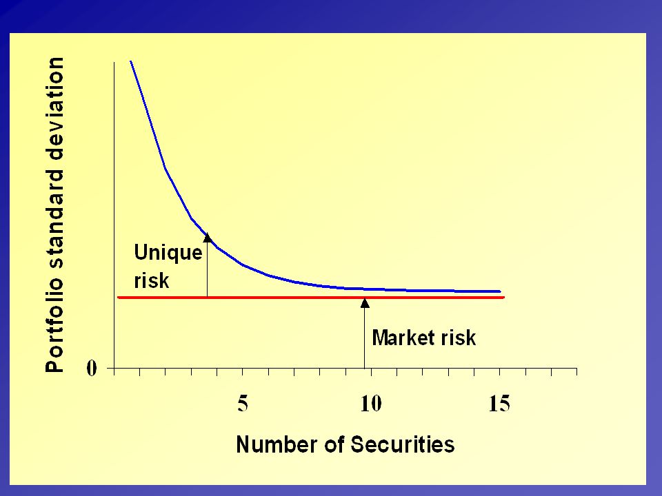
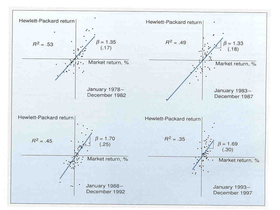
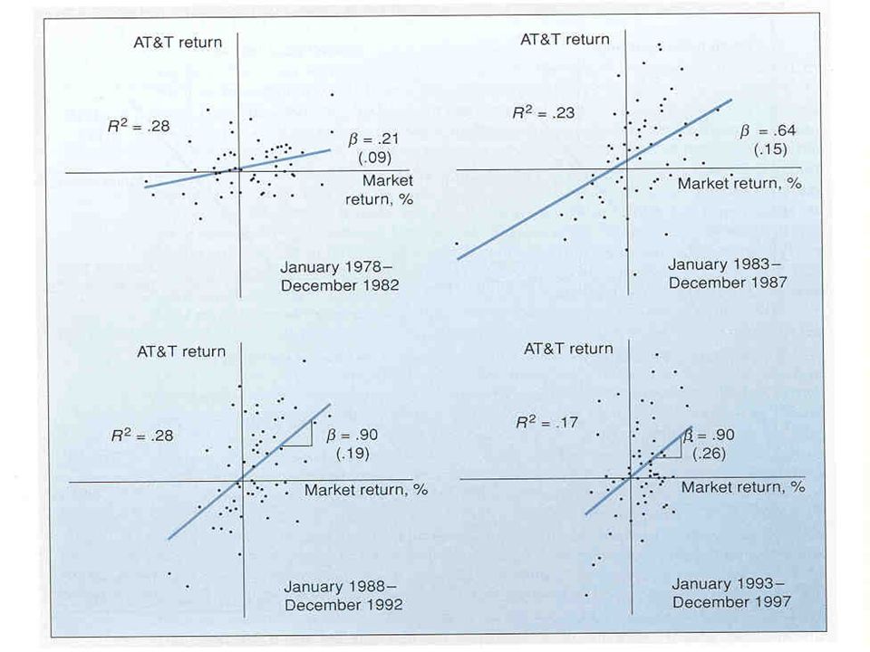
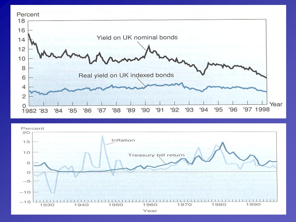
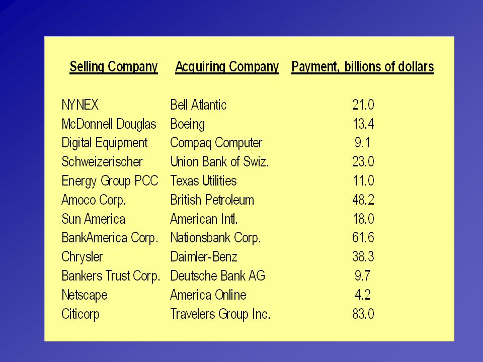
 Debt-holders are limited to a.>")


 “The firm`s mix of securities(long.>")
