Download presentation
Presentation is loading. Please wait.

1
Supervision Systems Design
Prof. Belkacem OULD BOUAMAMA Research Director Ecole Polytechnique de Lille Head of the research group “Bond Graphs” «LAGIS UMR CNRS8219» Laboratory Avenue Paul Langevin, F59655 Villeneuve d'Ascq cedex Tel : +33(0) , GSM: +33(0)
 , GSM: +33(0)")
2
PLAN Supervision software's Synthesis of monitoring systems
Supervision : Introduction and definitions Supervision software's Synthesis of monitoring systems Structural analysis and bipartite graph Information redundancy for FDI Observers for FDI LFT Bond graphs for robust FDI Design of supervision system. Application to a industrial systems Conclusions and bibliography

3
Part 1: Introduction

4
Bibliography Blanke, M., Kinnaert, M., Lunze, J. and Staroswiecki, M. (Eds)(2007) Diagnosis and Fault-Tolerant Control, Berlin:Springer-Verlag. "Automatique et statistiques pour le diagnostic". T1 et 2 sous la direction de Bernard Dubuisson, Collection IC2 Edition Hermes, 204 pages, Paris 2001. A.K. Samantaray and B. Ould Bouamama "Model-based Process Supervision. A Bond Graph Approach" . Springer Verlag, Series: Advances in Industrial Control, 490 p. ISBN: , Berlin 2008. D. Macquin et J. Ragot : "Diagnostic des systèmes linéaires", Collection Pédagogique d'Automatique, 143 p., ISBN X, Hermès Science Publications, Paris, 2000. B. Ould Bouamama, M. Staroswiecki and A.K. Samantaray. « Software for Supervision System Design In Process Engineering Industry ». 6th IFAC, SAFEPROCESS, , pp Beijing, China. B. Ould Bouamama, K. Medjaher, A.K. Samantary et M. Staroswiecki. "Supervision of an industrial steam generator. Part I: Bond graph modelling". Control Engineering Practice, CEP, Vol 1 14/1 pp 71-83, Vol 2. 14/1 pp 85-96, 2006. B. Ould-Bouamama. Contrôle en ligne d'une installation de générateur de vapeur par Bond Graph. Techniques de l'Ingénieurs AG pages 2014 B. Ould-Bouamama. La conception intégrée pour la surveillance robuste des systemes. Approche Bond Graph. Techniques de l'Ingénieurs AG pages 2013 R.Merzouki, A.K.Samantaray, M.Pathak and B. Ould-Bouamama. Intelligent Mechatronic Systems: Modelling, Control and Diagnosis. Springer Verlag, ISBN: , 943 pages, 2013. PhD Thesis, several lectures can be doownloaded at : //

5
Publications and co publications in the BG and FDI domain
BG theory BG for Modelling Bg for Supervision mechatronics Conseil d’Evaluation et d’Orientation DCSD (Commande des Systèmes Dynamiques et Commande du Vol) Théses : France Ahmed 7, Rochdi : 3, JY 4 , GDT 11, BOB : 9 Etranger Rochdi : 2 (Singapour), GDT : 1, BOB : 6 FDI software LFT BG Intelligent transport
 Théses : France Ahmed 7, Rochdi : 3, JY 4 , GDT 11, BOB : 9. Etranger Rochdi : 2 (Singapour), GDT : 1, BOB : 6. FDI software. LFT BG. Intelligent transport.")
6
Aims Acquire the methodological and practical knowledge on development and implementation of online monitoring systems (detection and isolation of faults) Understanding and acquire the structural analysis methodology for integrated design of complex systems supervision Understanding how online monitoring systems (SCADA system) can be developed and implemented Understanding the links between maintenance, control, on-line diagnosis, reconfiguration and analysis of operating modes and criticality
 Understanding and acquire the structural analysis methodology for integrated design of complex systems supervision. Understanding how online monitoring systems (SCADA system) can be developed and implemented. Understanding the links between maintenance, control, on-line diagnosis, reconfiguration and analysis of operating modes and criticality.")
7
What is a supervision : two levels FDI FTC?
Set of tools and methods used to operate an industrial process in normal situation as well as in the presence of failures. Supervision (IFAC): Monitoring a physical system and taking appropriate actions to maintain the operation in the case of faults. Activities concerned with the supervision : Fault Detection and Isolation (FDI) in the diagnosis level, and the Fault Tolerant Control (FTC) through necessary reconfiguration, whenever possible, in the fault accommodation level. SUPERVISION FDI : How to detect and to isolate a faults ? FTC : How to continue to control a process ?
: Monitoring a physical system and taking appropriate actions to maintain the operation in the case of faults. Activities concerned with the supervision : Fault Detection and Isolation (FDI) in the diagnosis level, and the Fault Tolerant Control (FTC) through necessary reconfiguration, whenever possible, in the fault accommodation level. SUPERVISION. FDI : How to detect and to isolate a faults FTC : How to continue to control a process")
8
Supervision Graphical User Interface (GUI)
Monitoring of variables (Data acquisition)? Surveillance (Alarms) Control
 Surveillance (Alarms) Control.")
9
Role of GUI (IHM) Synoptique fonction essentielle de la supervision,
fournit une représentation synthétique, dynamique et instantanée de l'ensemble des moyens de production de l'unité permet à l'opérateur d'interagir avec le processus et de visualiser le comportement normal Courbes: donne une représentation graphique de différentes données du processus Historisation du procédé: - permet la sauvegarde périodique de grandeurs (archivage au fil de l'eau) - permet la sauvegarde d'événements horodatés (archivage sélectif) - fournit les outils de recherche dans les données archivées - fournit la possibilité de refaire fonctionner le synoptique avec les données archivées ( fonction de magnétoscope ou de replay) - permet de garder une trace validée de données critiques (traçabilité de données de production) Gestion des Alarmes
 - permet la sauvegarde d événements horodatés (archivage sélectif) - fournit les outils de recherche dans les données archivées. - fournit la possibilité de refaire fonctionner le synoptique avec les données archivées. ( fonction de magnétoscope ou de replay) - permet de garder une trace validée de données critiques (traçabilité de données de. production) Gestion des Alarmes.")
10
Fonction of supervision systems
Management ERP : Enterprise Resource planning : planning of resources integration of different business functions in a centralized computer system configured according to the client-server mode. MRP : Manufacturing Resource Planning : planning of production Planning system which determines the component requirements from requests of finished products and existing suppliesPRODUCTION Process SCADA : Supervisory Control & Data Acquisition PC & PLC Process Control/ Programmable Logic Controller Supervisor A system that performs supervision by means of fault detection and isolation, determination of remedial actions, and execution a corrective actions.

11
Supervision and Monitoring
A continuous real time task of determining the conditions of a physical system, by recording information recognising and indicating anomalies of the behaviour (local security) Automatic control Control of parameters (to maintain the quality of products) Supervision Centralize monitoring and control tasks Two parts of SCADA system hardware (collect of datas) Software (control, display, monitoring)
 Automatic control. Control of parameters (to maintain the quality of products) Supervision. Centralize monitoring and control tasks. Two parts of SCADA system. hardware (collect of datas) Software (control, display, monitoring)")
12
Supervision in the hierarchy of a manufacturing company

13
Global Function of the supervision

14
Supervision softwares
Les logiciels de supervision sont une classe de programmes applicatifs dédiés à la production dont les buts sont : - l'assistance de l'opérateur dans ses actions de commande du processus de production (interface IHM dynamique...) - la visualisation de l'état et de l'évolution d'une installation automatisée de contrôle de processus , avec une mise en évidence des anomalies (alarmes) - la collecte d'informations en temps réel sur des processus depuis des sites distants (machines, ateliers, usines...) et leur archivage - l' aide à l'opérateur dans son travail (séquence d'actions/batch , recette/receipe) et dans ses décisions (propositions de paramètres, signalisation de valeurs en défaut, aide à la résolution d'un problème ...) - fournir des données pour l'atteinte d'objectifs de production (quantité, qualité, traçabilité, sécurité...)
 - la visualisation de l état et de l évolution d une installation automatisée de contrôle de processus , avec une mise en évidence des anomalies (alarmes) - la collecte d informations en temps réel sur des processus depuis des sites distants (machines, ateliers, usines...) et leur archivage. - l aide à l opérateur dans son travail (séquence d actions/batch , recette/receipe) et dans ses décisions (propositions de paramètres, signalisation de valeurs en défaut, aide à la résolution d un problème ...) - fournir des données pour l atteinte d objectifs de production (quantité, qualité, traçabilité, sécurité...)")
15
Supervision softwares

16
Supervision softwares
Wonderware InTouch Wonderware InTouch is the world’s number one Human Machine Interface (HMI) , Used in over one-third of the world’s industrial facilities open and extensible solution that enables the rapid creation of standardized, reusable visualization applications and deployment across an entire enterprise. Extensible library with more than 500 graphical symbols to build the system.
 , Used in over one-third of the world’s industrial facilities. open and extensible solution that enables the rapid creation of standardized, reusable visualization applications and deployment across an entire enterprise. Extensible library with more than 500 graphical symbols to build the system.")
17
Supervision softwares
PANORAMA : Ergonomic HMI module for alarms and events, an operating unit of historical datas. SIMATIC WinCC (Siemens) Supervision system with scalable features for monitoring automated processes, provides a full SCADA functionality in Windows Totally Integrated Automation System : Engennering, Communication, Diagnosis, Safety, Security, Robustess
 Supervision system with scalable features for monitoring automated processes, provides a full SCADA functionality in Windows. Totally Integrated Automation System : Engennering, Communication, Diagnosis, Safety, Security, Robustess.")
18
Supervision softwares
DSPACE MATLAB-Simulink More used for fast prototyping based on RealTime Interface (RTI) Residuals Simulink model RTI
 Residuals. Simulink model. RTI.")
19
How to select SCADA systems
Simplicity, Usability Solvers Image processing (icons, libraries, …) Supervision Control Surveillance Alarm processing Archiving Programing Performances/Price : Price : hardware + Operating system, software, support, documentation
 Supervision. Control. Surveillance. Alarm processing. Archiving. Programing. Performances/Price : Price : hardware + Operating system, software, support, documentation.")
20
Supervision system Architecture
Réseau d’entreprise Postes de Supervision Réseau d’atelier (Ethernet) Réseau de terrain (Profibus, Modbus, Asi…) Terminal d’atelier Automate (PID, TOR…) Capteurs Actionneurs Opérateur
 Réseau de terrain (Profibus, Modbus, Asi…) Terminal. d’atelier. Automate. (PID, TOR…) Capteurs. Actionneurs. Opérateur.")
21
Part 2: Objectives and definitions

22
Definitions Safety (sûreté) Security (sécurité)
Ability of a system to dispose of its functional performance (reliability, maintainability, availability) and not to cause a danger for persons or equipment or environment Safety is rather protection against accidental events. Security (sécurité) The condition of being protected from or not exposed to danger. Security is rather protection against intentional damages. Example : Aircraft security is about protecting the aircraft and it's contents from criminal activity and terrorism (Control of documents) Aircraft safety is about protecting the people by making the aircraft less likely to be involved in a crash (maintenance…)
 and not to cause a danger for persons or equipment or environment. Safety is rather protection against accidental events. Security (sécurité) The condition of being protected from or not exposed to danger. Security is rather protection against intentional damages. Example : Aircraft security is about protecting the aircraft and it s contents from criminal activity and terrorism (Control of documents) Aircraft safety is about protecting the people by making the aircraft less likely to be involved in a crash (maintenance…)")
23
Somme definitions Fault Failure (Défaillance) Types of fault
Unpermitted deviation of at least one characteristic property or parameter of the system from acceptable / usual / standard condition Incipient fault (naissante): A fault where the effect develops slowly e.g. clogging of a valve). In opposite to an abrupt fault. Abrupt fault : A fault where the effect develops rapidly (e.g. a step function). In opposite to an incipient fault. Active fault- tolerant system : A fault-tolerant system where faults are explicitly detected and accommodated. Contrary to a passive fault-tolerant system. Failure (Défaillance) Permanent interruption of a systems ability to perform a required function under specified operating conditions incipient failures (naissantes), Having a transitory nature constants Evolving over time catastrophic Types of fault
: A fault where the effect develops slowly e.g. clogging of a valve). In opposite to an abrupt fault. Abrupt fault : A fault where the effect develops rapidly (e.g. a step function). In opposite to an incipient fault. Active fault- tolerant system : A fault-tolerant system where faults are explicitly detected and accommodated. Contrary to a passive fault-tolerant system. Failure (Défaillance) Permanent interruption of a systems ability to perform a required function under specified operating conditions. incipient failures (naissantes), Having a transitory nature. constants. Evolving over time. catastrophic. Types of fault.")
24
Somme definitions Fault detection : Fault diagnosis: Fault isolation :
Determination of faults present in a system and time of detection Fault diagnosis: Determination of kind, size, location, and time of occurrence of a fault. Includes fault detection, isolation and identification Fault isolation : Determination of kind, location, and time of detection of a fault. Follows fault detection. Fault modeling : Determination of a mathematical model to describe a specific fault effect. Fault-tolerance : The ability of a controlled system to maintain control objectives, despite the occurrence of a fault. A degradation of control performance may be accepted. Fault-tolerance can be obtained through fault accommodation or through system and /or controller reconfiguration. Fault-tolerant system : A system where a fault is accommodated with or without performance degradation, but a single fault does not develop into a failure on subsystem or system level. Sensor fusion Integration of correlated signals from different sensors (information sources) into a single representation or action.
 into a single representation or action.")
25
Somme definitions Fault accommodation Disturbance: Perturbation:
(1) - A correcting action that prevents a certain fault to propagate into an undesired end-effect. (2) - Change in controller parameters or structure to avoid the consequences of a fault. The original control objective is achieved although performance may degrade. Disturbance: An unknown (and uncontrolled) input acting on a system Perturbation: An input acting on a system which results in a temporary departure from current state Constraint: The limitation imposed by nature (physical laws) or man. It permits the variables to take certain values in the variable space. Decision logic The functionality that determines which remedial action(s) to execute in case of a reported fault and which alarm(s) shall be generated. Detector An algorithm that performs fault detection and isolation
 - A correcting action that prevents a certain fault to propagate into an undesired end-effect. (2) - Change in controller parameters or structure to avoid the consequences of a fault. The original control objective is achieved although performance may degrade. Disturbance: An unknown (and uncontrolled) input acting on a system. Perturbation: An input acting on a system which results in a temporary departure from current state. Constraint: The limitation imposed by nature (physical laws) or man. It permits the variables to take certain values in the variable space. Decision logic. The functionality that determines which remedial action(s) to execute in case of a reported fault and which alarm(s) shall be generated. Detector. An algorithm that performs fault detection and isolation.")
26
Somme definitions Analytical redundancy Hardware redundancy
Use of more than one not necessarily identical ways to determine a variable, where one way uses a mathematical process model in analytical form. Hardware redundancy Use of more than one independent instrument to accomplish a given function. Availability: Probability that a system or equipment will operate satisfactorily and effectively at any point of time. MTTR: Mean Time To Repair MTTR = 1/µ; µ: rate of repair Reliability: Ability of a system to perform a required function under stated conditions, within a given scope, during a given period of time. Measure: MTBF = Mean Time Between Failure. MTBF = 1\la; la is rate of failure [e.g. failures per year]

27
Somme definitions : Models
Qualitative model A system model describing the behavior with relations among system variables and parameters in heuristic terms such as causalities or if-then rules. Qualitative equation Equations whose functional form and coefficient values are not completely specified. Quantitative model A system model describing the behavior with relations among system variables and parameters in analytical terms such as differential or difference equations. Residual Fault information carrying signals, based on deviation between measurements and model based computations. Threshold Limit value of a residual's deviation from zero, so if exceeded, a fault is declared as detected Symptom Change of an observable quantity from normal behaviour

28
Introduction From 1840: automatic control (Watt regulator)
Task: improve the quality of finished products, from 1980, new Challenge : Supervision Rôles : Provide the human operator assistance in its emergency management tasks alarm situations to increase the reliability, availability and dependability of the process. Apparition of integrated automation Control, diagnosis, optimization …

29
Integrated automation
FDI, FTC, aided decision tools Supervision level 3 Monitoring the state of the process, user interface level 2 Monitoring Control, optimisation Regulation level 1 Instrumentation Selection and implementation of sensors and actuators level 0 Decisions Observations Input Outputs

30
Relation between FDI et FTC Perf=F(Y1,Y2)
Hazardous area Hazardous Area UNACCEPTABLE PERFORMANCES DEGRADED PERFORMANCES Degraded performances Required Performances Fault Reconfiguration Y1

31
SUPERVISION in INDUSTRY
Set points Sensors y x u ur Controllers Actuator Process FTC Level Fault accommodation Reconfiguration FDI Level On line Fault Detection and isolation List of faulty components Corrective maintenance (after fault occurs)
")
32
Supervision system : different steps

33
FDI Purpose Objectives : given I/O pair (u,y), find the fault f . It will be done in 3 steps : DETECTION detect malfunctions in real time, as soon and as surely as possible : decides whether the fault has occured or not ISOLATION find their root cause, by isolating the system component(s) whose operation mode is not nominal : find in which component the fault has occured DIAGNOSIS diagnose the fault by identifying some fault model : determines the kind and severity of the fault
 whose operation mode is not nominal : find in which component the fault has occured. DIAGNOSIS. diagnose the fault by identifying some fault model : determines the kind and severity of the fault.")
34
FDI: Medical interpretaion
0 T 37 + - NON OUI Clinical examination (DETECTION) Diagnosis (ISOLATION)
 Diagnosis (ISOLATION)")
35
FDI steps in technological process supervisions
Detection : Is it really a fault ? Alarms generation Datas from Actual process Model + - isolation : Which component is faulty ? DECISION List of faulty components Technical specifications Identification : What is the type of fault? DIAGNOSIS Type of failures

36
FT (Fault Tolerance) and FTC (Fault Tolerant Control)
Analysis of fault tolerance : The system is runing under faulty mode Since the system is faulty, is it still able to achieve its objective(s) ? Design of fault tolerance : The goal is to propose a system (hardware architecture and sofware which will allow, if possible, to achieve a given objective not only in normal operation, but also in faulty situations. Control and Fault Tolerant Control Control algorithms : implement the solution of control problems : according to the way the system objectives are expressed FTC algorithms implements the solution of control problems : controls the faulty system the system objectives have to be achieved, in spite of the occurence of a pre-specified set of faults
 Design of fault tolerance : The goal is to propose a system (hardware architecture and sofware which will allow, if possible, to achieve a given objective not only in normal operation, but also in faulty situations. Control and Fault Tolerant Control. Control algorithms : implement the solution of control problems : according to the way the system objectives are expressed. FTC algorithms. implements the solution of control problems : controls the faulty system. the system objectives have to be achieved, in spite of the occurence of a pre-specified set of faults.")
37
Control Problem Traditional control : two kinds of objectives
control of the system , estimation of its variables Problematic : Given a set U of a control law ( open loop, closed loop, continuous or discrete variables, linear or non-linear) a set of control objective(s) O, set of uncertain constraints C(), (dynamic models) The solution is completely defined by the triple <O,C(), U >
 a set of control objective(s) O, set of uncertain constraints C(), (dynamic models) The solution is completely defined by the triple <O,C(), U >")
38
FTC problem FTC Controls the faulty system: 2 cases
1) fault adaptation, fault accommodation, controller reconfiguration change the control law without changing the system 2) system reconfiguration change both the control and the system : The difference with Control problem System constraints may change. Admissible control laws may change.
 fault adaptation, fault accommodation, controller reconfiguration. change the control law without changing the system. 2) system reconfiguration. change both the control and the system : The difference with Control problem. System constraints. may change. Admissible control laws. may change.")
39
Passive and active fault tolerance
Passive fault tolerance Active fault tolerance control law unchanged when faults occur specific solution for normal and faulty mode Normal mode Control law solves < O, Cn(n), Un > Faulty mode Control law also solves < O, Cf(f), Uf > f F <O,Cn(n),Un > and < O, Cf(f), Uf > f F Knowledge about Cf(f) and Uf must be available . FDI layer must give information. ROBUST TO FAULTS
, Un > Faulty mode. Control law also solves < O, Cf(f), Uf > f F. <O,Cn(n),Un > and. < O, Cf(f), Uf > f F. Knowledge about Cf(f) and Uf must be available . FDI layer must give information. ROBUST TO FAULTS.")
40
Fault accommodation and System reconfiguration
FDI system solve < O, f(f), Uf > Provide estimation of f(f), Uf of the fault impact Fault Provide estimation of Cf(f) Uf of the fault impact solve < O, Cf(f), Uf > Fault FDI cannot provide any estimation of the fault impact solve < O, Cr(r), Ur > Fault System reconfiguration Fault accommodation
, Uf > Provide estimation of. f(f), Uf of the fault impact. Fault. Provide estimation of. Cf(f) Uf of the fault impact. solve < O, Cf(f), Uf > Fault. FDI cannot provide. any estimation of the fault impact. solve < O, Cr(r), Ur > Fault. System. reconfiguration. Fault accommodation.")
41
Fault accommodation Fault FDI Accommodation Supervision Controller
parameters FDI Supervision Ref. Controller Process u Y Control system

42
Fault Reconfiguration
New control configuration Reconfiguration FDI Supervision Yref Nominal Controller Process Y u u' New Controller Y’ref Y’ Control system

43
Part 3: HOW TO DESIGN SUPERVISION SYSTEMS ?

44
DIAGNOSTIC METHODS (2/2)
Suivant le niveau de connaissance du processus à surveiller, on distingue deux grands types de méthodes de surveillance : Métode sans modèle : On ne dispose pas de modèles de comportement. On va donc les "apprendre" à partir de données expérimentales relevées dans les différents types de fonctionnement. On utilise les méthodes d'apprentissage Exemple diagnostic médical Méthode avec modèle : Dans ce cas on compare le comportement réel (fourni par des capteurs) au comportemnt temporel théorique fourni par les équations du modèle. Estimation des paramétres : Les données de la base de données brutes sont utilisées pour identifier les paramétres caractérisant le fonctionnemnr réel ; ceux ci sont comparées aux pâramétres théoriques Estimation d'état : Les données de la base de données brutes sont utilisées pour estimer les sorties du système qui sont comparées aus sorties réelles Redondance analytique : Les données de la base de données brutes sont injectées dans le modèle . Toute défaillance se traduit par par le fait que le modèle n'est pas vérifiéest alors
 au comportemnt temporel théorique fourni par les équations du modèle. Estimation des paramétres : Les données de la base de données brutes sont utilisées pour identifier les paramétres caractérisant le fonctionnemnr réel ; ceux ci sont comparées aux pâramétres théoriques. Estimation d état : Les données de la base de données brutes sont utilisées pour estimer les sorties du système qui sont comparées aus sorties réelles. Redondance analytique : Les données de la base de données brutes sont injectées dans le modèle . Toute défaillance se traduit par par le fait que le modèle n est pas vérifiéest alors.")
45
MODEL OF THE NORMAL OPERATION
Model-based FDI MODEL OF THE NORMAL OPERATION S E N SO R S Process actual operation ALARM GENERATION RESIDUAL GENERATOR ALARM INTERPRETAION Detection Isolation Identification

46
FDI based on Identification and observer
identification based y U + Residual - y Modèle Observer based y Observateur U Residual + -

47
No model based Pattern recognition methods ? ? ?
Determination of a set of classes (learning step) For each class is associated an operating mode (normal and faulty) Advantage Methods : statistical learning, data analysis, pattern recognition, neuronal networks, etc. Only experimental data are exploited No complex analytical model ? ? Problems need historical data in normal and in abnormal situations, every fault mode represented ??? generalisation capability ?? ?
 For each class is associated an operating mode (normal and faulty) Advantage. Methods : statistical learning, data analysis, pattern recognition, neuronal networks, etc. Only experimental data are exploited. No complex analytical model. Problems. need historical data in normal and in abnormal situations, every fault mode represented generalisation capability")
48
Example : FDI of a valve 1) No model based * +
Q P2 2) On line surveillance step 1) Pattern recognition step (classification of different modes) * D1 + D2 Flow Q(t) Pressure difference Pr = P1-P2
 On line surveillance step. 1) Pattern recognition step (classification of different modes) * D1. + D2. Flow. Q(t) Pressure difference Pr = P1-P2.")
49
QUALITATIVE METHODS Use expert knowledge based on « If then else » :
applying models of human thinking to physical systems Example : « If P1 increase then Q increase, else valve is blocked» advantage of qualitative methods: No need of numerical value of parameters neither deep knowledge of the system système. Easy to be implemented Issue Sensor faults not detected Lower and upper values of the deviation cannot be fixed precisely Combinatory problem can appear for complex systems (multivariable)
")
50
Model based : example Step 1 determination of fault indicator offline)
Q P2 Analytical model, parameters Step 1 determination of fault indicator offline) Residual signal Threshold
 Residual signal. Threshold.")
51
Steps in FDI system (1/4) 1. DETECTION
Logic operation : We state the system is faulty or not Criteria No detection or too late detection ➽ Catastrophic consequences for the process False alarms ➽ Unnecessary stops of the production unit. There are 4 hypothesis H0 : Assumption of normal operation (Decision domain D0) H1 : Assumption of faulty mode operation (Decision domain D0) Dx : No decision domain
 H1 : Assumption of faulty mode operation (Decision domain D0) Dx : No decision domain.")
52
Steps in FDI system (2/4) Problematic What to do ?
Given R=[r1, ….rn] fault indicators Two distributions are known p(Z/H0) and p(Z/H1) One of two hypotheses, H0 or H1 is true What to do ? Verify if each ri (i=1,..n) belongs to p(Z/H0) and p(Z/H1) 4 possibilités
 and p(Z/H1) One of two hypotheses, H0 or H1 is true. What to do Verify if each ri (i=1,..n) belongs to p(Z/H0) and p(Z/H1) 4 possibilités.")
53
Steps in FDI system (4/4) 2. ISOLATION 3. IDENTIFICATION (DIAGNOSIS)
To be able to isolate the failed components (Alarm filtering) using logic operations Criteria No isolability ➽ Catastrophic consequences for the process False isolability ➽ Unnecessary stops of the production unit or equipment. 3. IDENTIFICATION (DIAGNOSIS) When the fault is located, it is then necessary to identify the specific causes of this anomaly. Are the used logic operation based on signatures identified by experts and validated through expertise and repair faults.
 using logic operations. Criteria. No isolability ➽ Catastrophic consequences for the process. False isolability ➽ Unnecessary stops of the production unit or equipment. 3. IDENTIFICATION (DIAGNOSIS) When the fault is located, it is then necessary to identify the specific causes of this anomaly. Are the used logic operation based on signatures identified by experts and validated through expertise and repair faults.")
54
Technical specifications
Which parameters must be supervized ? What are the non acceptable values ? Objectives Performances false alarm missed detection detection delay Specifications Available data other (cost, complexity, memory, ...) Constraints
 Constraints.")
55
Logic Diagnosis : Systems and faults (1)
A system is a set of interconnected components A system is a triplet (SD, COMPS, OBS) SD : System Description, COMPS : Set of components OBS: set of observations COMPS = {comp1, comp2, comp3, comp4, comp5} x a b c d y z e f comp1 comp2 comp3 comp4 comp5
 SD : System Description, COMPS : Set of components. OBS: set of observations. COMPS = {comp1, comp2, comp3, comp4, comp5} x. a. b. c. d. y. z. e. f. comp1. comp2. comp3. comp4. comp5.")
56
COMPS = {input valve, tank, output pipe, level sensor}
System (2) COMPS = {input valve, tank, output pipe, level sensor} Continuous Hydraulic system SD Discrete electronic system x = a b y = b z = c d e = x y f = z ( y) x a b c d y z e f comp1 comp2 comp3 comp4 comp5
 COMPS = {input valve, tank, output pipe, level sensor} Continuous Hydraulic system. SD. Discrete electronic system. x = a b. y = b. z = c d. e = x y. f = z ( y) x. a. b. c. d. y. z. e. f. comp1. comp2. comp3. comp4. comp5.")
57
SM (or SD) is the set of all those constraints
System (4) SM (or SD) is the set of all those constraints Input valve Tank Output pipe Level sensor
 SM (or SD) is the set of all those constraints. Input valve. Tank. Output pipe. Level sensor.")
58
Examples of internal faults (1)
y b OK(comp2) is false x a b c d y z e f comp1 comp2 comp3 comp4 comp5
 is false. x. a. b. c. d. y. z. e. f. comp1. comp2. comp3. comp4. comp5.")
59
Examples of internal faults (2)
Actuator fault : input valve is blocked open Process fault : the tank is leaking Sensor fault : noise has improper statistical characteristics

60
Examples of external faults (2)
b c d y z e f comp1 comp2 comp3 comp4 comp5 a = 2 !! (it should equal to 1) Controller Control algorithm objective : cannot be achieved for too large output flows
 Controller. Control algorithm objective : cannot be achieved for too large output flows.")
61
SD is now ... Diagnosis algorithm OK(comp1) x = a b
OK(comp2) y = b OK(comp3) z = c d OK(comp4) e = x y OK(comp5) f = z ( y) SD is now ... OK(input valve) OK(tank) OK(output pipe) OK(level sensor)
 y = b. OK(comp3) z = c d. OK(comp4) e = x y. OK(comp5) f = z ( y) SD is now ... OK(input valve) OK(tank) OK(output pipe) OK(level sensor) ")
62
How to check the consistency
Problems Problem statement 1) For some given S COMPS, how to check the consistency of SD {OK(X)X S} OBS 2) How to find the collection of the NOGOODS How to check the consistency
 For some given S COMPS, how to check the consistency of. SD {OK(X)X S} OBS. 2) How to find the collection of the NOGOODS. How to check the consistency.")
63
Two means to check consistency
Analytical Redundancy properties that OBS should satisfy if actual system healthy properties that are satisfied by the nominal system trajectories check whether they are true or not Observers values that OBS should have if actual system healthy simulate / reconstruct the nominal system trajectories check whether they coincide with actual system trajectories

64
Chap.2 : ANALYTICAL REDUNDANCY

65
Model of the healthy system
Representation Model of the healthy system PROCESS Capteurs qp d x0 x(t) y(t) u(t) qm Model of the faulty system qm s qp x0 d p y(t) u(t) x(t) Capteurs PROCESS
 y(t) u(t) qm. Model of the faulty system. qm. s. qp. x0. d. p. y(t) u(t) x(t) Capteurs. PROCESS.")
66
State space representation
Linear case Disturbances Faults Disturbances Nonlinear case Faults

67
When the system is faulty ?
Given a system The system works in normal regime (hypothesis H0) means : y is produced according law C and x is produced according law f and is produced according law of probability P The system works in failure mode hypothesis H1) means : y is not produced according law C, or x is not produced according law f, or is not produced according law of probability P
 means : y is produced according law C. and x is produced according law f. and is produced according law of probability P. The system works in failure mode hypothesis H1) means : y is not produced according law C, or. x is not produced according law f, or. is not produced according law of probability P.")
68
Analytical redundancy :How to generate ARRS ?
Given The ARR express the difference between information provided by the actual system and that delivered by its normal operation model What is Residual ? All variables are known r u y

69
Analytical Redundancy Relations (ARR) and Residuals (r)
Definition ARR ARR is a mathematical model where all variables are known. The known variables are available from sensors, set points and control signal. ARR : F(u,x0, y, ) Residual r Residual is the numerical value of ARR (evaluation of ARR) R is a signal, ARR is an expression R= Eval (ARR) Problematic : How to generate ARRs ? Issue : Elimination of unknown variables theory
 Residual r. Residual is the numerical value of ARR (evaluation of ARR) R is a signal, ARR is an expression. R= Eval (ARR) Problematic : How to generate ARRs Issue : Elimination of unknown variables theory.")
70
General principle Analytic model measurement equations or
state and measurement equations Off-line Elimination of unknown variables techniques On-line Computation of ARRs (actual system)
")
71
Hardware and analytical redundancy
Hardware redundancy Detection Isolation Sensors F1 R S1 or S2 S2 S3 S2 S1 F2 Analytical redundancy ? Signature Fault Matrix (SFM) Leakage S1 F1 Valve R F2 r1 r2 1 1
 Leakage. S1. F1. Valve R. F2. r1. r")
72
Detectability and isolability
Fault Signature Matrix (FSM) Ib1 Ib2 … Ibm Mb1 Mb2 Mbm E1 E2 Em ARR1 S11 S12 S1m ARR2 S21 S22 S2m . ARRn Sn1 Sn2 Snm DEFINITION Ej (j=1,m) : Fault which may affect the jth component Sij : boolean value (0,1) Ib : Isolability Mb: Detectability
 Ib1. Ib2. … Ibm. Mb1. Mb2. Mbm. E1. E2. Em. ARR1. S11. S12. S1m. ARR2. S21. S22. S2m. . ARRn. Sn1. Sn2. Snm. DEFINITION. Ej (j=1,m) : Fault which may affect the jth component. Sij : boolean value (0,1) Ib : Isolability. Mb: Detectability.")
73
Detectability and isolability
The signature vector VEj (j=1,m) of each component fault Ej is given by the column vector: Detectability A component fault Ej is detectable (Mbj=1) if at least one sij (j=1,m) of its signature vector VEij is different than zero Isolability A component fault Ej is isolable (Ibj=1) if it is detectable and its signature vector VEij is different from others .
 of each component fault Ej is given by the column vector: Detectability. A component fault Ej is detectable (Mbj=1) if at least one sij (j=1,m) of its signature vector VEij is different than zero. Isolability. A component fault Ej is isolable (Ibj=1) if it is detectable and its signature vector VEij is different from others .")
74
Detectability and isolability example
Faults and ARR Fault Signature Matrix (FSM) Ib 1 Mb F1 S1 Leak. Valve R F2 ARR1 ARR2 Signature vectors Hamming Distance C: Binary coherence vector Sj : Signature vector of the jth component to be monitored to isolate k failures, the distance should be equal to 2k + 1.
 Ib. 1. Mb. F1. S1. Leak. Valve R. F2. ARR1. ARR2. Signature vectors. Hamming Distance. C: Binary coherence vector. Sj : Signature vector of the jth component to be monitored. to isolate k failures, the distance should be equal to 2k + 1.")
75
Hamming Distance The Hamming distance shows the ability to isolate two faults. Hamming distance (example) Signature vectors Hamming Distance of given example F1 S1 Leak. Valve R F2 1 2

76
Hardware redundancy : Simplest redundancy
Hardware redundancy uses only measurement equations (therefore it can detect only sensor faults) Example : duplex redundancy Model : y1 = x y2 = x Static ARR : y1 - y2 = 0
 Example : duplex redundancy. Model : y1 = x. y2 = x. Static ARR : y1 - y2 = 0.")
77
Duplex redundancy + - r t Max threshold Min threshold r1 Sensor 1 m1
Process Noised signal r1 Sensor 1 m1 Low pass filter m1f Alarms Alarm generator Variable x + - Noised signal Low pass filter m2f Sensor 2 m2 r2 r t Max threshold Min threshold Alarm Fn. normal

78
Triplex redundancy r1 = m1f - m2 f r2 = m1f – m3f Residuals
Thresholds m1 m1f Low pass filter Sensor 1 r1 Residual generation Decision procedure Alarms m2 Variable x m2f r2 Sensor 2 Low pass filter m3 r3 m3f Low pass filter Sensor 3 r1 t r2 r3 Residuals r1 = m1f - m2 f r2 = m1f – m3f r3 = m2f – m3f

79
Fault detection : three steps
y1 y2 Sensors acquisition Residual generation r = y1 - y2 + - Residual evaluation = 0 ? yes no

80
Fault detection : Problematic
y1 - y2 = 0 it is not impossible (but it is not certain) that both sensors are healthy Why is it so ??? because there might be non detectable faults
 that both sensors are healthy. Why is it so because there might be non detectable faults.")
81
Redundancy with Non detectable faults
Given fault model Computation form Evaluation form y1 = x + f1 y2 = x + f2 r = y1 - y2 = f1 - f2 r = 0 even when there is a combination of faults f1 and f2 such that : f1 - f2 = 0 Example : common mode failures non detectable faults

82
Redundancy with uncertainties
yes is never true y1 y2 = 0 ? Residual Generation r no is always true because y1 = x + 1 y2 = x + 2 r = y1 - y2 = 1 - 2 we need a model of the uncertainties Assume we know 1 [a1, b1], 2 [a2, b2], then we know 1 - 2 [a12, b12]

83
Redundancy with noises
y1 = x + 1 y2 = x + 2 r = y1 - y2 = 1 - 2 Assume we know P(1) and P(2), then we know P(1 - 2) is r distributed according to P(1 - 2) ??? r P(1 - 2) d(1 - 2) we need a Statistical decision theory r
 and P(2), then we know P(1 - 2) is r distributed according to P(1 - 2) r. P(1 - 2) d(1 - 2) we need a Statistical decision theory. r.")
84
How to isolate the fault ?
triplex redundancy y1 = x y2 = x y3 = x two residuals r1 = y1 - y2 = 0 r2 = y2 - y3 = 0 Remarks * any linear combination of residuals is a residual (r3 = y2 - y3) The set {r1, r2} is a residual basis in the following sense :
 The set {r1, r2} is a residual basis in the following sense :")
85
Fault isolation (fault model)
Triplex redundancy y1 = x + f1 x = y1 - f1 y2 = x + f2 x = y2 - f2 y3 = x + f3 x = y3 - f3 y1 - f1 = y2 - f2 y2 - f2 = y3 - f3 r1 = y1 - y2 = f1 - f2 r2 = y2 - y3 = f2 - f3 Computation form Evaluation form

86
Structured and directional residuals Directional residuals
Fault isolation Structured and directional residuals r1 = y1 - y2 = f1 - f2 r2 = y2 - y3 = f2 - f3 f1 f2 f3 r r Directional residuals En réponse à une défaillance donnée, le vecteur de résidus reste dans une direction spécifiée, propre à cette défaillance. En réponse à une défaillance donnée, certaines composantes (spécifiques à cette défaillance) du vecteur de résidus sont nulles.
 du vecteur de résidus sont nulles.")
87
Conclusion about hardware redundancy
detect sensor faults (if detectable) isolate sensor faults (if enough redundancy) needs noise models for statistical decision needs uncertainty models for set theoretic based decision powerful approach but multiplies weight and costs limited to sensor faults
 isolate sensor faults (if enough redundancy) needs noise models for statistical decision. needs uncertainty models for set theoretic based decision. powerful approach but multiplies weight and costs. limited to sensor faults.")
88
Static Analytical redundancy

89
Parity Space Given linear system Static redundancy d: fault,
Suppose m>n : Then, a decomposition of matrix C can be given under following form as : Such that C1 is inversible then measurement equation y(t) can be written : d: fault, Ԑ: uncertainties
 can be written : d: fault, Ԑ: uncertainties.")
90
Parity Space Then unknown variable X is calculated from y1,
and eliminated by replacing x(t) in Y2 : we obtain an ARR Evaluation and calculation form can be obtained
 in Y2 : we obtain an ARR. Evaluation and calculation form can be obtained.")
91
Parity space approach Then
Parity space approach to eliminate unknown variable x (Chow 84). : Find an orthogonal matrix W to C such that (WC=0) by multiplying measurement equation y=CX by W : Then The system of measurement equation is overdertermined w.r.t. to x : We have m-n ARR, while W has m-n linearly independent rows
. : Find an orthogonal matrix W to C such that (WC=0) by multiplying measurement equation y=CX by W : Then. The system of measurement equation is overdertermined w.r.t. to x : We have m-n ARR, while W has m-n linearly independent rows.")
92
Static Parity space Given measurement equation :
Columns of C : vector subspace of dimension R(C) : we note CR(C) Given additional subspace to CR(C) noted Wm-R(C) Wm-R(C) is named parity space Thus : CR(C) Wm-R(C)=Rm ( sum of vector space)
 : we note CR(C) Given additional subspace to CR(C) noted Wm-R(C) Wm-R(C) is named parity space. Thus : CR(C) Wm-R(C)=Rm ( sum of vector space)")
93
Projection of measurement equation onto parity space
ARR: in the absence of faults and disturbances (d(k)=f(k)=0) =0 Calculation form Evaluation form
=f(k)=0) =0. Calculation form. Evaluation form.")
94
Forms of vector parity Calculation form Evaluation form

95
Hardware redundancy based on substitution
Example : triplex redundancy y1 = x + f1 x = y1 - f1 y2 = x + f2 x = y2 - f2 y3 = x + f3 x = y3 - f3 r1 = y1 - y2 = f1 - f2 r2 = y2 - y3 = f2 - f3 y1 - f1 = y2 - f2 y2 - f2 = y3 - f3

96
Hardware redundancy based on parity space
ARR generation using parity space Parity space of dimension 2. Then a basis W can be choosen WC=0 (2 vectors orthogonal to C). Among those solutions, Parmi toutes les solutions choisissons : Projection of Y(t) onto parity space gives:
. Among those solutions, Parmi toutes les solutions choisissons : Projection of Y(t) onto parity space gives:")
97
Directional residuals
r(k) can be expressed as : Dimension of the parity space is 2. The direction of the residual vector depends on the specific direction of each fault. r1 r2 f1 f2 f3
 can be expressed as : Dimension of the parity space is 2. The direction of the residual vector depends on the specific direction of each fault. r1. r2. f1. f2. f3.")
98
Example of static redundancy
Given parity space u y2 y1 x1 x2 y3 To eliminate x, one find W such that : Wy = WCx = 0

99
Example of static redundancy
Residuals are : While dim(W)=1x3, then W = (a b c) All vectors under form : W= [a a] cancels WC One find thus the hardware redundancy:
=1x3, then W = (a b c) All vectors under form : W= [a 0 -a] cancels WC. One find thus the hardware redundancy:")
100
Conclusion about hardware redundancy
There is a static redundancy if one can find : A set of vectors W orthogonal to C such that : WC = 0 Row vectors of W define parity space : Projection of measurement equation onto parity space gives : Static ARR: W.Y = W.C.X = 0 Hardware redundancy concerns only sensor FDI Widely used in industry

101
A bit more complex Analytical redundancy (dynamic)
")
102
Dynamic Analytical Redundancy
State space model Continuous time Discrete time If there exists W such that WC = 0 then static redundancy relations can be found

103
Dynamical Analytical redundancy (continuous)
Differenciation of y

104
Dynamical Analytical redundancy (Discrete)
Differenciation of y

105
Analytical redundancy (dynamic)
If there exists W such that W then

106
Analytical redundancy (general)
Dérivation de y Observability matrix OBS(A, C, p) Toeplitz matrix T(A, B, C, D, p) Dérivation de y(n)
 Toeplitz matrix. T(A, B, C, D, p) Dérivation de y(n)")
107
Expressions of dynamical ARRs
If there exists W such that ARRs are : Rows of W are a basis of Ker(OBS), define the parity space Parity space dimension is number of sensors
, define the parity space. Parity space dimension is number of sensors.")
108
RESUME REDONDANCE DYNAMIQUE
Given the system At time K+1 Using (1) we have Then: generalizing until the order p (1) (2) (3) (4)
 we have. Then: generalizing until the order p. (1) (2) (3) (4)")
109
Fault detection Computation form Evaluation form = 0 when no fault
0 when fault is present

110
Cayley-Hamilton Theorem
Consequence of Cayley-Hamilton Theorem It exists order p such that rank of OBS(A,C,p) matrix is smaller than the number of rows : thus we can find a matrix W such that : W.OBS(A,C,p) = 0 Additional space to OBS, defined by W, is named « Parity space ». By projection of measurement equation (3) onto this space, we obtain: Dynamic ARR : The residual is
 matrix is smaller than the number of rows : thus we can find a matrix W such that : W.OBS(A,C,p) = 0. Additional space to OBS, defined by W, is named « Parity space ». By projection of measurement equation (3) onto this space, we obtain: Dynamic ARR : The residual is.")
111
Application Derivation up to second order
Calcul W : derivation first order : CB D

112
Application We fix arbitrarily 2 unknowns
Find two linearly independent vectors W We fix arbitrarily 2 unknowns W3 is linear combination of W1 and W2 Residuals expressions are then :

113
Application If r=0, we obtain initial model

114
Second order residual Matrices OBS and T will be :
We obtain after claculation Analysis 2nd order residual (cf r4) is sensible only to Y2 (Good for isolation) If the order is increased, are obtained the same ARRS but time shifted RRAs (filtered) 2nd order Residual 1st order residual (obtained before)
 is sensible only to Y2 (Good for isolation) If the order is increased, are obtained the same ARRS but time shifted RRAs (filtered) 2nd order Residual. 1st order residual (obtained before)")
115
Conclusions detects any fault (if detectable)
isolates any fault (if enough redundancy) estimates the unknown variable with several estimation versions needs noise models for statistical decision needs uncertainty models for set theoretic based decision
 estimates the unknown variable with several estimation versions. needs noise models for statistical decision. needs uncertainty models for set theoretic based decision.")
116
CHAP3: Structural Analysis
Motivations Structural description Structural properties Matching Causal interpretation of matchings Subystems characterization System decomposition Conclusion

117
Motivations Complex systems : hundreds of variables and equations
Many different configurations Many different kinds of models (qualitative, quantitative, static, dynamic, rules, look-up tables, …) Description of physical plants as interconnected subsystems Analytic models not available The structural description of a system expresses only the links between the variables and the constraints Structural analysis Analysis of the structural properties of the models, i.e. properties that are independent on the actual values of the parameter.
 Description of physical plants as interconnected subsystems. Analytic models not available. The structural description of a system expresses only the links between the variables and the constraints. Structural analysis. Analysis of the structural properties of the models, i.e. properties that are independent on the actual values of the parameter.")
118
Graphs : some definitions
A graph is an ordered pair G = (V, E) which consists of a set V of vertices or nodes together with a set E of edges or lines A graph is used to specify relationships among a collection of items. The are Simple (undirected graphs) and oriented (directed) graphs Examples social networks, in which nodes are people or groups of people, and edges represent some kind of social interaction Communication networks : computers are nodes, and the edges represent direct links along which messages can be transmitted. A A C D C D B B Undirected (simple) Graph Directed (oriented) Graph (A points to B but not vice versa
 which consists of a set V of vertices or nodes together with a set E of edges or lines. A graph is used to specify relationships among a collection of items. The are Simple (undirected graphs) and oriented (directed) graphs. Examples. social networks, in which nodes are people or groups of people, and edges represent some kind of social interaction. Communication networks : computers are nodes, and the edges represent direct links along which messages can be transmitted. A. A. C. D. C. D. B. B. Undirected (simple) Graph. Directed (oriented) Graph (A. points to B but not vice versa.")
119
Digraph: definitions The digraph ? [Blanke and al. 2003]
Given the state equation The digraph ? [Blanke and al. 2003] Graph whose set of vertices corresponds to the set of inputs ui, output yj and state variables xk Edges are defined as : An edge exists from vertex xk (respectively from vertex ul ) to vertex xj if and only if the state variable xk (respectively the input variable ul ) really occurs in the function F (i.e. vertex ui ) in the function An edge exists from vertex xk to vertex yj if and only if the state variable xk really occurs in the function g Physical means Digraph is a structural abstraction of the behaviour model where Edges represent mutual influence between variables : The time evolution of the derivative xi depends to the time evolution of xk
![Digraph: definitions The digraph [Blanke and al. 2003]](http://slideplayer.com/slide/4239498/14/images/119/Digraph%3A+definitions+The+digraph+%5BBlanke+and+al.+2003%5D.jpg "Given the state equation. The digraph [Blanke and al. 2003] Graph whose set of vertices corresponds to the set of inputs ui, output yj and state variables xk. Edges are defined as : An edge exists from vertex xk (respectively from vertex ul ) to vertex xj if and only if the state variable xk (respectively the input variable ul ) really occurs in the function F (i.e. vertex ui ) in the function. An edge exists from vertex xk to vertex yj if and only if the state variable xk really occurs in the function g. Physical means. Digraph is a structural abstraction of the behaviour model where. Edges represent mutual influence between variables : The time evolution of the derivative xi depends to the time evolution of xk.")
120
Directed graph representation
Means : the time evolution of the derivative depends to the time evolution of x2 Directed graph representation Edge represents mutual influence between variables (x1 influences y y x1 u x2

121
Structural description
Behaviour model of a system : a pair (C, Z) Z = {z1, z2,...zN } is a set of variables and parameters, C = {c1, c2,...cM } is a set of constraints Variables quantitative, qualitative, fuzzy Constraints algebraic and differential equations, difference equations, rules, etc. time continuous, discrete
 Z = {z1, z2,...zN } is a set of variables and parameters, C = {c1, c2,...cM } is a set of constraints. Variables. quantitative, qualitative, fuzzy. Constraints. algebraic and differential equations, difference equations, rules, etc. time. continuous, discrete.")
122
Structure of controlled system
Cc Cp Cm X Y U Yref Controller Process Sensor + - S=(C,Z) C : set of constraints Z : set of variables U, subset of control variables Y, subset of measured variables X, subset of unknown variables Structure = binary relation S : C x Z {0, 1} (ci, zj) S(ci, zj)
 C : set of constraints. Z : set of variables. U, subset of control variables. Y, subset of measured variables. X, subset of unknown variables. Structure = binary relation. S : C x Z {0, 1} (ci, zj) S(ci, zj)")
123
Bipartite graph A graph is bipartite if its vertices can be partitioned into two disjoint subsets C and Z such that each edge has one endpoint in C and the other one in Z. Bi-partite graph : links between variables and constraints

124
Definition The structural model of the system (C,Z) is a bipartite graphe (C,Z,A) , Where A is a set of edges defined as follows : Example C Z C1 C2 i y u

125
Example bipartite graph (1)
ue uC C0 uR i uL R0 um L0 Remark ! In some papers are introduced 2 additional constraints (differential) and corresponding variables to express just the derivative of variable:
 and corresponding variables to express just the derivative of variable:")
126
Example : bipartite graph (2)
Z C um c1 c2 c3 c4 c5 ue uL uC uR i K=known variables X=Unknown variables Cardinal = size (dimension) of a vector
 of a vector.")
127
Example : bipartite graph (3)
The differential constraints could be added Z C c1 c2 c3 c4 c5 c6 c7 um ue uL uC uR i z1 z2 Differential constraints and variables

128
Incidence matrix A bipartite graph can be represented by an adjacency matrix (named incidence matrix). This is a Boolean matrix where each row corresponds to a constraint ci and each column to a variable zj. A “1” at position (i, j) indicates that there is an edge connecting the constraint ci and the variable zj. Variables Z UnKnown variables Known variables The incidence matrix B is the matrix whose rows and column represent the set of constraints or variables, respectively. Every edge (ci, zj) is represented by « 1 » in the intersection of ci and zj. Constraints C
. This is a Boolean matrix where each row corresponds to a constraint ci and each column to a variable zj. A 1 at position (i, j) indicates that there is an edge connecting the constraint ci and the variable zj. Variables Z. UnKnown variables. Known variables. The incidence matrix B is the matrix whose rows and column represent the set of constraints or variables, respectively. Every edge (ci, zj) is represented by « 1 » in the intersection of ci and zj. Constraints C.")
129
Subsystem : definition
The Structure of a system is a bipartite graph G(C, Z, A) , where A is a set of edges such that : (c, z) C Z, a = (c, z) A the variable z appears in the constraint c Definition 2. The structure of a constraint c is a subset of variables Z(c) such that : z Z(c), (c, z) A Definition 3. A subsystem is a pair (, Z()) where is a subsystem of C and Z() = c Z(c).
 , where A is a set of edges such that : (c, z) C Z, a = (c, z) A the variable z appears in the constraint c. Definition 2. The structure of a constraint c is a subset of variables Z(c) such that : z Z(c), (c, z) A. Definition 3. A subsystem is a pair (, Z()) where is a subsystem of C and Z() = c Z(c).")
130
Example of a subsystem A subsystem is a pair (, Z()) where is a subset of C and Z() = c , Z(c). Subsystem (R,L) C/Z uR uL uC i um ue c1 1 c2 c3 c4 c5 C/Z uR uL i c1 1 c2
 C/Z. uR. uL. uC. i. um. ue. c1. 1. c2. c3. c4. c5. C/Z. uR. uL. i. c1. 1. c2.")
131
Differential and algebraic equations
Are used three kinds of equations: Differential Algebraic Measure Used variables are

132
Hydraulic example Tank dx(t)/dt - qi(t) + qo(t) = 0
Input valve c2: qi(t) - αu(t) = 0 Output pipe c3: q0(t) - kv(x(t)) = 0 Level sensor 1 c4: y1(t) - x(t) = 0 Level sensor c5: y2(t) - x(t) = 0 Output flow sensor c6: y3(t) - qo (t) = 0 Control algorithm y1 y2 U(t) qi y3 LC q0 x=volume c7: u(t) = 1 if lmin y1(t) lmax u(t) = 0 else
 - αu(t) = 0. Output pipe c3: q0(t) - kv(x(t)) = 0. Level sensor 1 c4: y1(t) - x(t) = 0. Level sensor 2 c5: y2(t) - x(t) = 0. Output flow sensor c6: y3(t) - qo (t) = 0. Control algorithm. y1. y2. U(t) qi. y3. LC. q0. x=volume. c7: u(t) = 1 if lmin y1(t) lmax. u(t) = 0 else.")
133
Bipartite graph and incidence matrix
c1: dx(t)/dt - qi(t) - qo(t) = 0 c2: qi(t) - αu(t) = 0 c3: q0(t) - kv(x(t)) = 0 c4: y1(t) - x(t) = 0 c5: y2(t) - x(t) = 0 c6: y3(t) - qo (t) = 0 c7: u(t) = 1 if lmin x(t) lmax u(t) = 0 else c1 c2 c3 c4 c5 c6 c7 x(t) qi(t) qo(t) u(t) y1(t) y2(t) y3(t)
/dt - qi(t) - qo(t) = 0. c2: qi(t) - αu(t) = 0. c3: q0(t) - kv(x(t)) = 0. c4: y1(t) - x(t) = 0. c5: y2(t) - x(t) = 0. c6: y3(t) - qo (t) = 0. c7: u(t) = 1 if lmin x(t) lmax. u(t) = 0 else. c1. c2. c3. c4. c5. c6. c7. x(t) qi(t) qo(t) u(t) y1(t) y2(t) y3(t)")
134
State space model and digraph
Digraph representation Bipartie graph representation

135
Subsystems A subsystem : Q(Ci) consists of 2 parts
is a pair (Ci, ,Q(Ci) where Q(Ci) is the set of variables constrained by constraints Ci Q(Ci) consists of 2 parts Qc(Ci): correspond to known variables and Qx(Ci): correspond aux unknown variables Example : Hydraulic system C1 Q(C1)
 where Q(Ci) is the set of variables constrained by constraints Ci. Q(Ci) consists of 2 parts. Qc(Ci): correspond to known variables and Qx(Ci): correspond aux unknown variables. Example : Hydraulic system. C1. Q(C1)")
136
Dulmage-Mendelsohn decomposition
The number of solutions for Qx(Ci) obtained from Qc(Ci) characterize each subsystem Any system can be uniquely decomposed into 3 subsystems : Over-constrained (C+,X+) Just-constrained (C0,X0) Under-constrained (C-,X-) Only the over-constrained subsystem is monitorable Example of overdetermined system C/Z x X-{x} y1 y2 f1 1 f2 c1 : F1(y1, x) = 0 c2: F2 (y2, x) = 0 x=(F2)-1 (y2) x=(F1)-1 (y1) Subsystem {c1, c2} overdetermines the unknown variable x : x can be computed via two different ways , The two results have to be identical
 obtained from Qc(Ci) characterize each subsystem. Any system can be uniquely decomposed into 3 subsystems : Over-constrained (C+,X+) Just-constrained (C0,X0) Under-constrained (C-,X-) Only the over-constrained subsystem is monitorable. Example of overdetermined system. C/Z. x. X-{x} y1. y2. f1. 1. f2. c1 : F1(y1, x) = 0. c2: F2 (y2, x) = 0. x=(F2)-1 (y2) x=(F1)-1 (y1) Subsystem {c1, c2} overdetermines the unknown variable x : x can be computed via two different ways , The two results have to be identical.")
137
Under determined subsystem
(C, Q(C)) is under determined if, For each value of known variable Qc(C), the set of unknown variables Qx(C) verifying the constraints C has a cardinal higher than one. : card(C)<card(Qx(C)) (number of equations less than number of variables) Causes : not enough equations to determine x variables Qx(C) cannot be calculated from known variables Qc(C) and constraints C. Result of insufficient modeling of the system, or non observability of certain variables.
) is under determined if, For each value of known variable Qc(C), the set of unknown variables Qx(C) verifying the constraints C has a cardinal higher than one. : card(C)<card(Qx(C)) (number of equations less than number of variables) Causes : not enough equations to determine x. variables Qx(C) cannot be calculated from known variables Qc(C) and constraints C. Result of insufficient modeling of the system, or non observability of certain variables.")
138
Just and over determined subsystems
(C, Q(C)) is just determined if : card(C)=card(Qx(C)) The unknown variables Qx(C) can be calculated uniquely from known variables Qc(C) and constraints C. (C, Q(C)) is over determined : card(C)>card(Qx(C)) Causes Variables Qx(C) can be calculated in different ways from the known variables Qc (C) and the constraints C Each subset Ci C provides a different way to calculate Qx (C). Since the results of these calculations are identical (they are the same physical variables), there are some analytical redundancy
) is just determined if : card(C)=card(Qx(C)) The unknown variables Qx(C) can be calculated uniquely from known variables Qc(C) and constraints C. (C, Q(C)) is over determined : card(C)>card(Qx(C)) Causes. Variables Qx(C) can be calculated in different ways from the known variables Qc (C) and the constraints C. Each subset Ci C provides a different way to calculate Qx (C). Since the results of these calculations are identical (they are the same physical variables), there are some analytical redundancy.")
139
Examples (1/2) y1 1 1 Z={X} U {K} y1 X={u, i}, K={y1,} C1: u-Ri=0
C2: y1-u=0 i R u y1 Subsystem : C1(i,u)=0 1 C1(i,u)=0 u i y1 C2(y1,U)=0 1 (C1, Q(C1)) is under determined Card(C1)=1<Card(Qx (C1)=2. (C2, Q(C2)) is juste determined : Card(C2)=1=Card(Qx (C2) (C, Q(C)) is juste détermined: Card(C)=2=Card(Qx (C)=2
=0. 1. C1(i,u)=0. u. i. y1. C2(y1,U)=0. 1. (C1, Q(C1)) is under determined. Card(C1)=1<Card(Qx (C1)=2. (C2, Q(C2)) is juste determined : Card(C2)=1=Card(Qx (C2) (C, Q(C)) is juste détermined: Card(C)=2=Card(Qx (C)=2.")
140
Example (2/2) y1 y2 1 1 i y1 y2 Z=XUK X={u, i}, K={y1, y2,} C1: U-Ri=0
C2: y1-u=0 C3: y2-i=0 1 y1 C2(y1,u)=0 C1(i,,u)=0 u i y2 C3(i,y2)=0 1 (C, Q(C)) is over determined: Card(C)=3>Card(Qx (C)=2
=0. C1(i,,u)=0. u. i. y2. C3(i,y2)=0. 1. (C, Q(C)) is over determined: Card(C)=3>Card(Qx (C)=2.")
141
Example : Incidence matrix
y2 x={u, i} K={y1} C1: U-Ri=0 C2: y1 –U=0 x={u, i} K={y1 ,y2,} C1: U-Ri=0 C2: y1 –U=0 C3: y2-U=0 x={u, i} K={} C1: U-Ri=0 i R u y1 C/Z u i C1(i,u)=0 y2 C3(u,y2)=0 1 y1 C2(y1,u)=0 1 1 1
=0. y2. C3(u,y2)=0. 1. y1. C2(y1,u)=")
142
Matching and ARRs

143
Definition of a matching
Consider the graph G(Cx, X, Ax), restriction of the structural graph of the system where Cx : Constraints related to unknown variables X Ax : set of edges linking Cx to X. Let a AX, We note X(a) the end of a in X and CX(a) extremity of a in CX. The edge can be written as : a = (Cx(a), X(a)) A A={a1, a2, …an) X={x1, x2, …xn) C={c1, c2, …cn) C X Cx(a) X a C(x) X(a)
, restriction of the structural graph of the system where. Cx : Constraints related to unknown variables X. Ax : set of edges linking Cx to X. Let a AX, We note X(a) the end of a in X and CX(a) extremity of a in CX. The edge can be written as : a = (Cx(a), X(a)) A. A={a1, a2, …an) X={x1, x2, …xn) C={c1, c2, …cn) C. X. Cx(a) X. a. C(x) X(a)")
144
Matching : Definition (1/2)
G(Cx, X, A) is a matching on G(Cx, X, Ax) if and only if 1) A Ax 2) a1, a2 A a1 a2 Cx(a1) Cx(a2) X(a1) X(a2) Interpretation A matching is : a set of pairs (ci,xi) s.t. the variable xi can be computed by solving the constraint ci, under the hypothesis that all other variables are known a1 X(a1) Cx(a1) X C(x) a2 X(a2) Cx(a2) X C(x)
 is a matching on G(Cx, X, Ax) if and only if. 1) A Ax. 2) a1, a2 A a1 a2. Cx(a1) Cx(a2) X(a1) X(a2) Interpretation. A matching is : a set of pairs (ci,xi) s.t. the variable xi can be computed by solving the constraint ci, under the hypothesis that all other variables are known. a1. X(a1) Cx(a1) X. C(x) a2. X(a2) Cx(a2) X. C(x)")
145
Matching : Definition (2/2)
A mathing is a subset of edges such that any two edges have non common node (neither in C nor in Z) Differents matchins can be defined on a bi-partite graph C1(i,,u)=0 C2(y1,u)=0 C3(i,y2)=0 Different matchings of unknown variables i i C1 C1 u u C2 C2 y1 y1 y2 y2 C3 C3
 Differents matchins can be defined on a bi-partite graph. C1(i,,u)=0. C2(y1,u)=0. C3(i,y2)=0. Different matchings of unknown variables. i. i. C1. C1. u. u. C2. C2. y1. y1. y2. y2. C3. C3.")
146
Maximal matching A maximal matching on G(Cx, X, Ax) is a matching G(Cx, X, A) s.t.: A' A, A' A G(Cx, X, A') is not a matching. What is it ? A maximal matching is a matching such that no edge can be added without violating the no common node property C1 C2 C3 i u y1 y2 This matching is maximal w.r.t X : Any matching can be added This matching is not maximal w.r.t X (C3,u) can be added i C1 u C2 y1 y2 C3
 can be added. i. C1. u. C2. y1. y2. C3.")
147
Complete and incomplete matching
A matching β is complete w.r.t to C (set of constraints ) respectively to X (set of variables) if : x X, c C such that (c,x) β : complete w.r.t. C c C, x X such that (c,x) β : complete w.r.t. X C1(i,,u)=0 C2(y1,u)=0 C3(u,y2)=0 This matching is incomplete w.r.t. to C (C3 is not matched) but complete w.r.t. to X C1(i,,u)=0 X C i i C1 C1 X (unknown variables) u u C2 y1 This matching is complete w.r.t. to C But incomplete w.r.t. to X K (known variables while measured) y2 C3
 respectively to X (set of variables) if : x X, c C such that (c,x) β : complete w.r.t. C. c C, x X such that (c,x) β : complete w.r.t. X. C1(i,,u)=0. C2(y1,u)=0. C3(u,y2)=0. This matching. is incomplete w.r.t. to C. (C3 is not matched) but complete w.r.t. to X. C1(i,,u)=0. X. C. i. i. C1. C1. X (unknown variables) u. u. C2. y1. This matching. is complete w.r.t. to C. But incomplete w.r.t. to X. K (known variables. while measured) y2. C3.")
148
Matching and the incidence matrix 1/2
Select at most one "1" in each row and in each column Each selected "1" represents an edge of the matching No other edge should contain the same variable : it is the only one in the row No other edge should contain the same constraint : it is the only one in the column.

149
Matching and the incidence matrix 2/2
C/Z u i y1 y2 y2 u C2(y1,u)=0 C1(u,i)=0 C3(u,y2)=0 1 C2 y1 y2 C3 C1 C2 C3 i u y1 y2 C/Z u i y1 y2 y2 C2(y1,u)=0 C1(u,i)=0 C3(u,y2)=0 1
=0. C1(u,i)=0. C3(u,y2)=0. 1. C2. y1. y2. C3. C1. C2. C3. i. u. y1. y2. C/Z. u. i. y1. y2. y2. C2(y1,u)=0. C1(u,i)=0. C3(u,y2)=0. 1.")
150
Causal interpretation of matchings
Causal graph ? The oriented bipartite graph which results from a causality assignment is named Causal graph Algebraic constraints At least one variable can be matched in a given constraint Non invertible algebraic constraints Consider C(x1,x2)=0 x1 x2 C Impossible matching C x1 x2 Possible matching C/Z x1 x2 C 1 C/Z x1 x2 C 1 x 1
=0. x1. x2. C. Impossible matching. C. x1. x2. Possible matching. C/Z. x1. x2. C. 1. C/Z. x1. x2. C. 1. x. 1.")
151
Oriented graph associated with a matching
Causal and acausal constraint u-Ri=0 : acausal constraint have not a direction. The variables have the same status: the graph is non oriented U = Ri : causal constraint : i is known, u is calculated. Here the matching is chosen. The matched constraint is associated with one matched variable and with some non matched one u i C C: u-Ri=0 Non matched constraint u i C: U=RI Matched constraint Oriented graph

152
Oriented graph associated with a matching
Matched constraints the output is computed : the inputs are supposed to be known. The edges adjacent to a matched constraints are oriented C/Z x x1 x2 x3 C1 1 C2 C3 C4 1 x1 C-1(x1,x2,x3) x x2 1 x3 1 1
 x. x2. 1. x")
153
Oriented graph associated with a matching
Non-matched constraints all the edges adjacent to a non-matched constraint are inputs. The relation C is redundant. All variables are inputs C/Z x1 x2 x3 C1 1 C2 C3 C4 x1 x2 x3 c1 Maximal matching w.r.t. to X But incomplete w.r.t. to C C1 is redundant (is not used to eliminate X) 1 1 1
")
154
Structural properties Diagnosability conditions

155
Structural observability
Under derivative causality, the system is structurally observable if and only if : 1. All the unknown variables are reachable from the known ones (measure) 2. the over constrained and just-constrained subsystems are causal (no differential loop) 3. the under-constrained subsystems is empty
 2. the over constrained and just-constrained subsystems are causal (no differential loop) 3. the under-constrained subsystems is empty.")
156
Over and just constrained system
The system is over-constrained if There is a causal matching which is complete w.r.t. all the unknown variables but not w.r.t. all the constraints. The unknown variables can be expressed (in several ways) as functions of the known variables. The subsystem is observable and redundant The system is just-constrained if : There is a causal matching which is complete w.r.t. all the unknown variables and all the constraints. The unknown variables can be expressed as functions of the known variables. The subsystem is observable
 as functions of the known variables. The subsystem is observable and redundant. The system is just-constrained if : There is a causal matching which is complete w.r.t. all the unknown variables and all the constraints. The unknown variables can be expressed as functions of the known variables. The subsystem is observable.")
157
Under-constrained system
The system is under-constrained if There is no causal matching which is complete w.r.t. the unknown variables. The subsystem is not observable, and not monitorable. Structural monitorability The conditions for a fault to be monitoable are : 1. the subsustem is observable 2. the fault belongs to the structurally observable over constrained part of the subsystemm to be monitored

158
Under and juste constrained system
C1: u-Ri=0 i R u y1 C1: u-Ri=0 C2: y1-u=0 i R ❷ Bipartite graph ❷ Bipartite graph i C1 i C1 u u C2 One solution (non redundancy) y1 No solution ❸ Oriented graph ❸ Oriented graph C1 C2 C1 y1 u i All constraints are used: there is no a redundancy Oriented graph
 y1. No solution. ❸ Oriented graph. ❸ Oriented graph. C1. C2. C1. y1. u. i. All constraints are used: there is no a redundancy. Oriented graph.")
159
Over constrained system (matching 1)
x={u, i}, K={y1 ,y2,} C1: U-Ri=0, C2: y1 –U=0, C3: y2-U=0 ❷ Bipartite graph and incidence matrix ❸ Oriented graph and ARR Maximal matching w.r.t. to X Incomplète matching w.r.t. to C C1 C2 y1 y2 C3 0 edge

160
Over constrained system (matching 2)
0 edge

161
Exercise y2 u y1 R i ❶ System ❷ Constraints
❸ Bipartite graph and incidence matrix ❹ Oriented graph and ARR

162
Alternated chain What is alternated chains ?
A path between two nodes (variables or constraints) alternates always successively variables and constraints nodes : this path is said alternated chain Lenth of alternated chain ? Number of constraints accrosed along the path Reachability A variable x1 is reachable from variable x2 if there exists an alternated chain from x1 to x2 Example Number of constraints : 2 Number of variables : 3 Lenth of alternated chain : 2 The variable i is reachable from y1 The path between i and y1 is : y1→C1 →u →C1 →i Nodes C2 C1 y1
 alternates always successively variables and constraints nodes : this path is said alternated chain. Lenth of alternated chain Number of constraints accrosed along the path. Reachability. A variable x1 is reachable from variable x2 if there exists an alternated chain from x1 to x2. Example. Number of constraints : 2. Number of variables : 3. Lenth of alternated chain : 2. The variable i is reachable from y1. The path between i and y1 is : y1→C1 →u →C1 →i. Nodes. C2. C1. y1.")
163
Hydraulic example : differential constraint
Graphe bipartite z y C1 qo V R C2 V qi C3 y y C4 qi C1 Zero C3 V C2 qo Maximal matching w.r.t. to X Incomplète matching w.r.t. to C Zero edge C4 z

164
Differential constraints
Differential constraints can always be represented under the form: x2 = dx1/ dt Derivative and integral causality Derivative causality Integral causality Initial conditions must be known

165
Loops Definitions Algebraic loop C1 1 C2 1 1
In the oriented graph, loops are a special subset of constraints, which have to be solved simultaneously, because the output signals of some constraints in the loop are the inputs are some others in the same loop : the number of matched variables is equal to the number of constraints (length of the loop). Algebraic loop C/Z x1 x2 C1 1 C2 C3 V C2 qo x2 C1 x1 1 1
. Algebraic loop. C/Z. x1. x2. C1. 1. C2. C3. V. C2. qo. x2. C1. x")
166
Differential loop: example
2) Using integral causality : there is one solution if initial condition is known V R V C2 qi C1 q0 1) Using derivative causality : there is no solution V C2 C4 qi C1 z q0 Differential loop
 Using integral causality : there is one solution. if initial condition is known. V. R. V. C2. qi. C1. q0. 1) Using derivative causality : there is no solution. V. C2. C4. qi. C1. z. q0. Differential loop.")
167
Differential loop How to broke the loop Adding a sensor
A matching without any differential loop is called a causal matching C3 y V C2 C4 qi C1 z q0

168
Example just-constrained system
Suppose input flow qi is unknown All unknown variables matched V C2 C4 C1 z q0 C3 y qi C/Z z=dV/dt V qi qo y C1 1 C2 C3 C4 1 1 All constraints are matched 1 1

169
Example Over-constrained system
All unknown variables matched C/Z z=dV/dt V qi qo y u C1 1 C2 C3 C4 C5 V C2 C4 C1 z q0 C3 y u C5 qi Redundancy 1 1 C1 is not matched 1 1

170
What is happened in integral causality?
X :All unknown variables matched C/Z V(0) V qi qo y u C1 1 C2 C3 C5 V C2 C1 q0 C3 y u qi V(0) C5 1 1 C : All constraintsare matched 1 1 The system is now just-determined : the matching is complete w.r.t to X and C.
 V. qi. qo. y. u. C1. 1. C2. C3. C5. V. C2. C1. q0. C3. y. u. qi. V(0) C C : All constraintsare matched The system is now just-determined : the matching is. complete w.r.t to X and C.")
171
Example under-constrained system
C/Z z=dV/dt V qi qo u C1 1 C2 C4 C5 The system is not observable There is a differential loop 1 V C2 C4 C1 z q0 u qi C5 1 1 1

172
Conclusions (1/2) Structural analysis based on bipartite graphs is easy to understand, easy to apply, Shows the relation between constraints and components, Allows to : identify the monitorable part of the system, i.e. the subset of the system components whose faults can be detected and isolated, Advantages Easy to implement and suited for complex systems Allows to determine the FDI/FTC possibilities No a priori knowledge of the model equations is necessary Lack Structural analysis produces only structural properties

173
Conclusiosn (2/2) :What we can do with structural analysis ?
can the system be observed ? can all the system variables be computed from the knowledge of the sensors outputs can the system be controlled ? can the system be monitored ? can the malfunction of the system components be detected and isolated can the system be reconfigured ? can the system achieve some objective in spite of the malfunction of some components Actual properties are only potential when structural properties are satisfied. They can certainly not be true when structural properties are not satisfied. Structural properties are properties which hold for actual systems almost everywhere in the space of their independent parameters

174
Chapter 3 : Observer-based approaches

175
Introduction Principle of FDI methods observer based Observer ?
Reconstruction of the output from sensor and comparison of this estimation with the real output In function of the system: deterministe case : estimation with observers Stochastic case : Kalman filter Observer ? Is a state reconstructor that from measured variables preform estimation of state vector Software sensor !

176
What is observer ? Given x y u Process C
How to reconstruct based on output error Process u x C y

177
Simulation of the observer
C A-KC

178
Observer and process A C + B PROCESS B K A C + - OBSERVER

179
Convergence (1/2) Convergence conditions
 Convergence conditions")
180
Convergence (2/2) Erreur d’estimation
s’annule exponentiellement si (A-KC) est asymptotiquement stable i.e. valeurs propres (modes) sont à partie réelles négatives : Comment ? : Bien choisir K
 est asymptotiquement stable i.e. valeurs propres (modes) sont à partie réelles négatives : Comment : Bien choisir K.")
181
Remarks Conclusion The reconstruction error is not zero because
The IC of the observer is choosen arbitraly and IC of the process are unknowns How to cacal the error: We can act only on K: then choose K to stabilize the matrix A-KC ensuring convergence to zero the error Used Techniques: Poles Placement used to set the speed of convergence by adjusting the coefficient K (see the instructions on Matlab place and acker

182
Idea of diagnosis based observer
Estimation error cannot be generated (the state is not measured) But : error of the recontructor can be calculated while Y is measured mesurée Scheme : Residual Process Observer Compare u
 But : error of the recontructor can be calculated while Y is measured mesurée. Scheme : Residual. Process. Observer. Compare. u.")
183
How to generate residuals ?
1. Par simulation + y C + process A-KC - y Residual + Sensor

184
Calculation of residual using z transform

185
Calcul du résidu en p L (1) (2)
 (2)")
186
Residual Using P transform (1)-(2) : Rsidual
Aprés quelques simplifications Lemme d’inversion de matrice : Residual

187
Convergence and sensitivity to the noise
Analysis of r(p) 1. The reconstruction error of the output depends on the estimation error of the CI 2. Dilemma between : convergence of the observer and the residue sensitivity to noise Choose the gain K so that the error converges rapidly (by imposing the eigenvalues of the matrix very low) : But if K becomes too sensitive to random noise residue
 1. The reconstruction error of the output depends on the estimation error of the CI. 2. Dilemma between : convergence of the observer and the residue sensitivity to noise. Choose the gain K so that the error converges rapidly (by imposing the eigenvalues of the matrix very low) : But if K becomes too sensitive to random noise residue.")
188
Example Simple monovariable case Convergence de l’erreur
Stability conditions

189
Simulation SIMULATION

190
Generalized Luenberger Observer
Given: 1. We want to estimate the output y(t) Is used observer of gain K X(t) : state, u(t) : input d(t) : faults e(t) : distubancess or noises (1) (2)
 Is used observer of gain K. X(t) : state, u(t) : input. d(t) : faults. e(t) : distubancess or noises. (1) (2)")
191
Erreurs estimation 2. Dynamic equations of the error estimation
(1)- (2) 3. Laplace trasnform of output error
- (2) 3. Laplace trasnform of output error.")
192
Remarks about the residual
Le résidue is sensitive to fault d(p), to disturbances and noises e(p), but also to the IC. Observation converge to 0 for t, we can neglect transitory due of CI. If d=0, e=0, we have the expression obtained previously.. The gain K of the observer affects similarly d and e: So it is difficult to generate a residual sensitive to faults but not to disturbances Analysis of matrices G indicates whether components are to be isolated from other
, to disturbances and noises e(p), but also to the IC. Observation converge to 0 for t, we can neglect transitory due of CI. If d=0, e=0, we have the expression obtained previously.. The gain K of the observer affects similarly d and e: So it is difficult to generate a residual sensitive to faults but not to disturbances. Analysis of matrices G indicates whether components are to be isolated from other.")
193
Different influences to the residue
1. Influence of the noise Let e(t) noise realization of a Esp (e (t) = 0 random variable Find the residue in frequential Using the above equations the terms of reconstruction errors are obtained (assuming D = 1 Ey = 0) Observer Fréquentiel
 noise realization of a Esp (e (t) = 0 random variable. Find the residue in frequential. Using the above equations the terms of reconstruction errors are obtained (assuming D = 1 Ey = 0) Observer. Fréquentiel.")
194
Influence of the noise to the residue
Négligeons d’abord l’influence des CI Etude de l’influence du point de vue fréquentiel de e sur r(p) Reduction of the noise e(jω) and r(jω) : Find a gain K, by placing the cut-off frequency of the filter such as the influence of noise is reduced
 Reduction of the noise e(jω) and r(jω) : Find a gain K, by placing the cut-off frequency of the filter such as the influence of noise is reduced.")
195
Calcul du seuil d’alarmes du résidu
Soit données les hypotheses statistiques du bruit : Consider the estimator If average noise e is null it is the same for the estimator

196
Calculation of the alarm threshold of the residue
Equation variance propagation Application to the error estimation

197
Calculation of the alarm threshold of the residue
Threshold in stationary regim Determine a threshold in the decision process of the presence of faults based on the variance of y beyond which the residue will be considered null (there is really an alarm) K V0 Détermination of variance of the residual t Threshold ALARM NORMAL
 K. V0. Détermination of variance of the residual. t. Threshold. ALARM. NORMAL.")
198
2. Influence d’une erreur de modélisation
Problematic In practice there is always a modeling error Observer built from the model, then the reconstructed output is sensitive to modeling errors Diagnosis is based on the difference between real and reconstructed output Difficult to separate due to modeling errors and those due to faults Goal Build an observer sensitive to faults and insensitive to modeling errors

199
Développement Let uncertain state model : consider error only on A Estimation of the state Cet observateur doit alors détecter, au travers de l’erreur de reconstruction de la sortie, la perturbation du système A Traduit l’apparition d’une perturbation A sur le système Représente un observateur calé sur le système nominal

200
Assumptions about the error
Error hypothesis Assumptions about the error Bounded : i.e slight inaccuracy of the model coefficients Problem to solve : générate residuals 1. less sensitive to A 2. with a maximum sensitivity to faults

201
Influence of parameter uncertainties
1. Influence of variations of A to the residues Error estimation (from previous equations) : Frequential domain The reconstruction error is sensitive to inaccuracies A and to the state x(t) (not eliminated here)
 : Frequential domain. The reconstruction error is sensitive to inaccuracies A and to the state x(t) (not eliminated here)")
202
Influence of input and A
Influence of input u to the resdiue For IC=0, and replacing x(p) by its expression we have : Then residue depends on u and A We exploit this property to distinguish the influences to the residue of faults and uncertainties How ? : While A is unknown , the error estimation is expressed in terms of what is applied (i.e. u) for (A ) we calculate the threshold for max A
 by its expression we have : Then residue depends on u and A. We exploit this property to distinguish the influences to the residue of faults and uncertainties. How : While A is unknown , the error estimation is expressed in terms of what is applied (i.e. u) for (A ) we calculate the threshold for max A.")
203
Decision Scheme of the decision procedure
U (bornée) Upper bound of the construction error (residue) If the residual value is below the threshold then diagnosis is reserved because the error may be due to uncertainties Beyond this threshold amplitude of the residue indicates the presence of a fault different from model errors t ALARM NORMAL
 Upper bound of the construction error (residue) If the residual value is below the threshold then diagnosis is reserved because the error may be due to uncertainties. Beyond this threshold amplitude of the residue indicates the presence of a fault different from model errors. t. ALARM. NORMAL.")
204
Unknown Input Observers (UIO)
Problematic Models where the output of the actuators is not measured Evaluation of RRAs requires knowledge measures and inputs So: is used unknown input observers (UIO: Unknown Input Observers) Principle Let a system with known inputs u(t) And unknown inputs
 Principle. Let a system with known inputs u(t) And unknown inputs.")
205
Observateur à entrée inconnue
Let system with UI Consider then the following observer : The error estimation will be :

206
Differentiating and substituting x (t) and z (t), then::
Let : P = I+EC

207
The reconstruction error of the state of the UIO
While the input is unknown, we try to have : This reconstruction tends then asymptotically to zero iff :

208
Calculation of UIO Procedure to calculate the UIO
Calculate the generalized inverse of CF Deduct P and G We fix the poles of N and then we deduce K and N L is calculated The unknown input is not involved in the expression of residue.

209
Estimation of UI Initial equation of the system :
If (CF)-1 exists we will have :
-1 exists we will have :")
210
Different UIO schemes SOS : Simplified Observer Scheme
Only one UIO Allows to detect faults. No isolation possibilities DOS : Dedicated Observer Scheme Bank of UIO Each observer is sensitive to one fault (diagonal structure)
")
211
D.O.S w.r.t. actuators u y Actuators System Sensors u1 umu UIO 1 e1
emu UIO mu Diagonal structure w.r.t. actuator faults

212
D.O.S w.r.t. sensors u y System Sensors Actuators umu e1 UIO 1 u1 emu
UIO mu Diagonal structure w.r.t. sensor faults

213
G.O.S w.r.t. actuators u y Actuators System Sensors u1 umu UIO 1 e1
emu UIO mu Each residual is affected by all faults except for one sensor fault

214
BOND GRAPH FOR ROBUST FDI

215
PLAN 1) Motivations et positionnement
2) Problématique des méthodes à base de modèles 3) Bond graph et le diagnostic 4) Conception d’un système de supervision 5) Outil logiciel pour la conception de systèmes de supervision 6) Application a un générateur de vapeur
 Problématique des méthodes à base de modèles. 3) Bond graph et le diagnostic. 4) Conception d’un système de supervision. 5) Outil logiciel pour la conception de systèmes de supervision. 6) Application a un générateur de vapeur.")
216
Contexte Résultats de recherche depuis 12 ans
B. Ould Bouamama and A.K. Samantaray. "Model-based Process Supervision. A Bond Graph Approach" . Springer Verlag, To be published on 2007, Berlin. Thoma J.U. et B. Ould Bouamama. "Modeling and Simulation in Thermal and Chemical Engineering". A Bond Graph Approach. Springer Verlag, 219 pages, Berlin 2000. More : Web : Applications Projet Européens (CHEM, damadics) supervision de procédés chimiques et pétrochimiques, raffinerie de sucre , .. Projet nationaux : EDF Filtrage d’alarmes Projet régional : supervision de procédés non stationnaires Outils logiciels développés Model Builder « FDIPAD » Génération de modèles et d’indicateurs de fautes formels à partir des PIDs Analyse de la surveillabilité : placement de capteurs Génération de S-function ou code C pour la simulation La supervision aujourd’hui dans l’industrie
 supervision de procédés chimiques et pétrochimiques, raffinerie de sucre , .. Projet nationaux : EDF Filtrage d’alarmes. Projet régional : supervision de procédés non stationnaires. Outils logiciels développés. Model Builder « FDIPAD » Génération de modèles et d’indicateurs de fautes formels à partir des PIDs. Analyse de la surveillabilité : placement de capteurs. Génération de S-function ou code C pour la simulation. La supervision aujourd’hui dans l’industrie.")
217
Integrated design for supervision
New sensor architecture Optimal sensor placement Diagnosability results Technical specifications Diagnosability analysis ARRs Uncertain Parameters P&ID Process Generate a dynamic and formal models Generate a formal and robust ARRS Online implementation Data from sensors Sensors

218
Conception intégrée de systèmes pilotés : Démarche
Thème 3 Informatisation Placement de Capteurs et actionneurs Propriétés structurelles et causales Commandabilité, Observabilité Surveillabilité, Reconfigurabilité Simplification de modèles Thème 2 Propriétés formelles et comportementales Indicateurs de fautes formels Dimension-nement Synthèse de lois de commande Thème 2 Thème 1 Test en ligne

219
Pourquoi les BGs pour la conception intégrée
Pourquoi les BGs pour la conception intégrée ? Graphes et Bond Graphs : quelles différences ?

220
Génération automatique des modèles

221
Why Graphical Approach for integrated design?
Graphical methods that are based essentially on structural models Graph structures independent of the numerical values of the syst. parameters. Structural properties are independent of the values of the system Structural description of a system expresses only the links between the variables and the constraints Visualization of the system topology Many different kinds of models linear, non linear can be used (qualitative, quantitative, static, dynamic, rules, look-up tables, …) Lack Structural analysis produces only structural properties
 Lack. Structural analysis produces only structural properties.")
222
State of art BOND GRAPH For MODELLING (1959)
Control (Vergé, Gawtrop, Dauphin, Sueur, Rahmani..) 1991 Diagnosis Sizing Qualitative approach (1993) Linkens, Mosterman, Kohda, .. Quantitative approche (1995) Opend loop system Linear Systems Sensor and actuator Faults Monoenergy Bond Graph (Tagina 95) Hybrid Bond Graph (Biswas, Mosterman (USA) Coupled BG (Ould Bouamama 198) Robust Diagnosis Extension to coupled BG Automated Diagnosis Design of supervision system 222
 Diagnosis. Sizing. Qualitative approach (1993) Linkens, Mosterman, Kohda, .. Quantitative approche (1995) Opend loop system. Linear Systems. Sensor and actuator Faults. Monoenergy Bond Graph (Tagina 95) Hybrid Bond Graph (Biswas, Mosterman (USA) Coupled BG (Ould Bouamama 198) Robust Diagnosis. Extension to coupled BG. Automated Diagnosis. Design of supervision system")
223
Model based approach : Issues
MODELLING Modelling step is most important in FDI design obtaining the model is a difficult task The constraints are not deduced in a systematic way It is not trivial in the real systems to write the model under a "beautiful" form x=f(x,u,θ). RESIDUAL GENERATION Eliminate the unknowns : analytic redundancy approach Existing methodology : parity space for linear, elimination theory (constraints under polynomial forms) Variables to be considered : all quantities constrained by the system components (process, actuators, sensors, algorithms) How to generate directly from the process ARRs and models : Bond graph tool well suited because of its causal and structural properties.
. RESIDUAL GENERATION. Eliminate the unknowns : analytic redundancy approach. Existing methodology : parity space for linear, elimination theory (constraints under polynomial forms) Variables to be considered : all quantities constrained by the system components (process, actuators, sensors, algorithms) How to generate directly from the process ARRs and models : Bond graph tool well suited because of its causal and structural properties.")
224
DEFINITION, REPRESENTATION
2 1 Mechanical power : REPRESENTATION P = e.f e f

225
Notion de causalités

226
POWER VARIABLES FOR SEVERAL DOMAINS
Electrical DOMAIN Mechanical (rotation) Hydraulic Chemical Thermal Economic Mechanical (translation) FLOW (f) EFFORT (e) VOLTAGE u [V] CURRENT i [A] FORCE F [N] VELOCITY v [m/s] TORQUE [Nm] ANGULAR VELOCITY [rad/s] PRESSURE P [pa] VOLUME FLOW CHEM. POTENTIAL [J/mole] MOLAR FLOW TEMPERATURE T [K] ENTROPY FLOW UNIT PRICE Pu [$/unit] FLOW OF ORDERS fc [unit/period]
 Hydraulic. Chemical. Thermal. Economic. Mechanical (translation) FLOW (f) EFFORT (e) VOLTAGE. u [V] CURRENT. i [A] FORCE. F [N] VELOCITY. v [m/s] TORQUE. [Nm] ANGULAR VELOCITY. [rad/s] PRESSURE. P [pa] VOLUME FLOW. CHEM. POTENTIAL. [J/mole] MOLAR FLOW. TEMPERATURE. T [K] ENTROPY FLOW. UNIT PRICE. Pu [$/unit] FLOW OF ORDERS. fc [unit/period]")
227
T2 On-Off Vo QO PI T1

228
T1 T2 1 1 C:C1 C:C1 R:R1 R:R1 Se1 MSf1 On-Off Vo PI QO USER u3 PI u1
Tank1 C:C1 De1 2 On-off Tank2 C:C1 De2 6 Valve1 1 R:R1 4 3 5 Valve 2 1 R:R1 Se1 7 8 9 Pump MSf1 1 T2 On-Off PI T1 Vo QO Outflow to consumer

229
Specialized software for Bond graph modelling

230
3) Bond graph and diagnostic : determinsit and robust case
 Bond graph and diagnostic : determinsit and robust case")
231
Bipartite graphs and Bond graphs
, The structural model of the system (C,Z) is a bipartite graphe (C,Z,A) The constraints C from the bond graph model consist of structural Cs, behavioral Cb and measurement equations Cm: The structural constraints are deduced from the set of junction equations which represent the mass and energy conservation laws. The number of junction equations is then equal to the number of equations in 0-junction (common effort), 1-junction (common flow) and 2-ports elements (transformer TF, gyrator GY):
 is a bipartite graphe (C,Z,A) The constraints C from the bond graph model consist of structural Cs, behavioral Cb and measurement equations Cm: The structural constraints are deduced from the set of junction equations which represent the mass and energy conservation laws. The number of junction equations is then equal to the number of equations in 0-junction (common effort), 1-junction (common flow) and 2-ports elements (transformer TF, gyrator GY):")
232
Measurement (Cm) equations represent the sensor equations
Behavior equations (Cb) describe the physical phenomena occurred in passive BG elements (Resistive R , Capacitive C and Inertial I): Measurement (Cm) equations represent the sensor equations De and Df are effort and flow detectors respectively. The set of variables The set of variables Z consists of known (K) and unknown (X) variables. The known variable set K contains the effort (Se) and flow (Sf) source variables : Unknown variables X are the pair of conjugated power variables (flow and effort):
 describe the physical phenomena occurred in passive BG elements (Resistive R , Capacitive C and Inertial I): Measurement (Cm) equations represent the sensor equations. De and Df are effort and flow detectors respectively. The set of variables. The set of variables Z consists of known (K) and unknown (X) variables. The known variable set K contains the effort (Se) and flow (Sf) source variables : Unknown variables X are the pair of conjugated power variables (flow and effort):")
233
Cardinality from BG model
Consider the jth junction structure (JS) where occur several phenomena represented by set of n bond graph elements E : E1, …Em To this junctions are connected m sensors : S1, …Sm This junction is completely defined by one structural equation (energy conservation) , n behavioral equations (how this energy is transformed) and m measurement equations.
 where occur several phenomena represented by set of n bond graph elements E : E1, …Em. To this junctions are connected m sensors : S1, …Sm. This junction is completely defined by one structural equation (energy conservation) , n behavioral equations (how this energy is transformed) and m measurement equations.")
234
The cardinal of unknown variables
The number of unknown variables in 0-junction is equal to the set of flow variables plus the common effort variable which links all elements Similarly on the 1-junction, the number of unknown variables is the sum of effort variables labeling the components bond graph plus the common flow variable General case, the unknown variables cardinal can be written by the relation: For global system Consider now the global bond graph model of the system to be monitored which consists of junctions . The cardinal of the unknown variables and the cardinal of constraints can be given through the following relations:

235
ARRs generation from Bond Graphs
ARR is a constraint calculated from over determined subsystem where all variables are known: In a bond graph representation ARR is

236
Covering causal path Définion (Causal path)
A causal path between two ports is an alternation of bonds and basic bond graph elements (named nodes) such that (i) all nodes have a correct and complete causality, and (ii) two bonds of the path have in the same node opposite causal stroke direction. Simple direct Causal path : covered following only one variable (effort or flow). Indirect causal path : one element (R,C, I) should be crossed along the path Mixad causal path : it comprises a gyrator (GY) imposing the change of followed variable e 1 f e 1 f Passive element (R, C, I e 1 GY f
 such that (i) all nodes have a correct and complete causality, and (ii) two bonds of the path have in the same node opposite causal stroke direction. Simple direct Causal path : covered following only one variable (effort or flow). Indirect causal path : one element (R,C, I) should be crossed along the path. Mixad causal path : it comprises a gyrator (GY) imposing the change of followed variable. e. 1. f. e. 1. f. Passive element (R, C, I. e. 1. GY. f.")
237
Causal path and causality
E C iC UC i F UC iC i C Se:E Derivative causality Sf: i Integral causality Se:E UC iC Sf:i UC i

238
How causal path can help for simulation !
Df:i UR R:R1 Df:i i UR ir R1 Uc E Uc E C Se:E 1 C:C1 ie ic g For 1 junction ❶ E Uc UR + - For R elemnt UR ir R:R1 For C element Uc ic C:C1 Df:i

239
Dualised sensors RL circuit
Se: u RL circuit Bond graph model in derivative causality with dualised sensor why ? Initial Conditions no knowns Df : as source of information I Se Df R Bond graph model in integral causality For control and simulation I SSf Df Se R

240
Pas de conflit de causalité, Système sur-déterminé
SSf SSf Df Df Se SSe Se De ? R R Pas de conflit de causalité, Système sur-déterminé Conflit de causalité, Système sous-Déterminé

241
Example a DC motor ua ia w ELECTRICAL PART MECHANICAL PART LOAD

242
Systematic State equations generation
ia m (J,f) La Ra im ua w 1 R:Ra I:La uM ia uRa uLa 1 L w I:J R:f Se:-L f J MSe:Ua ia ua MGY :K w Df:m Df:im
 La. Ra. im. ua. w. 1. R:Ra. I:La. uM. ia. uRa. uLa. 1. L. w. I:J. R:f. Se:-L. f. J. MSe:Ua. ia. ua. MGY. :K. w. Df:m. Df:im.")
243
Automated Control analysis

244
Algorithme de génération des RRAs à partir du modèle BG
❶ Put the BG model in derivative causality dualising sensors 1 R:Ra I:La uM ia uRa uLa 1 L w I:J R:f Se:-L f J MSe:Ua ia ua MGY :K w SSf:m SSf:im

245
Structural analysis Cardinal of constraints
Cardinal of Unknown variables

246
Incidence matrix and Bipartie graph of the Dc motor

247
❷ The structure junction (conservative law equation) associated with at least one sensor represents the candidate
 associated with at least one sensor represents the candidate")
248
❸ The unknown variables are eliminated using covering causal paths from unknwn to known variables (measured and control signal) 1 R:RA I:La uM ia uRa uLa 1 L w I:J R:RM Se:-L f J MSe:Ua ua MGY :K w SSf:m SSf:im

249
Oriented graph

250
Decision procedure: monitorability analysis
Ri/fautes L Re Ua Im Wm Jm Rm R1 1 R2

251
Decision procedure: monitorability analysis

252
Informatisation FDIPAD

253
Robustness problem

254
How to fix threshold ? Seuil simple: 3*std Fonctionnement normal
Défaut sur capteur du courant égal à 15% de sa valeur nominale

255
What about parameter uncertainties ?
introduction of 5% of nominal value of RM False alam because of parameter uncertainties !!!!

256
Linear Fractional Transformation
Any rational expression can be written under LFT form LFT Représentation State space representation LFT Representation Transfert Function used for stability analysis and for control law synthesis using the m-analysis and synthesis principles,

257
LFT Modelling R fR eR fR eR R fR eR δR eR einc Rn fR eRn
Mathematical model Modele bloc diagramme Physical system R fR eR fR eR R fR eR δR eR einc + Rn fR eRn

258
LFT modelling 1 R:Rn De*:zR MSe*:wR -δR eRn f1=fRn einc fR eR zR wR
R:Rn De*:zR MSe*:wR -δR eRn f1=fRn einc fR eR zR wR -δR eR R:R fR Rn fRn eRn eR + R fR eR + einc δR

259
Example R:Rn R:R Se: u I:L I:Ln De*:zR MSe:wR Df: i Se: u Df*:zL
2 5 9 6 R:R 2 R L i A Se: u 4 1 Se: u Df: i I:Ln 3 10 MSf:wL 7 Df*:zL 8 3 I:L

260
ARR generation : determinist (1/1)
2 1 4 1- Se Se: u 1 Df: i SSf: i SSf- 2-R-2 3 SSf- 3- L- 3 I:L R L i A Se: u

261
R:Rn Se: u I:Ln De*:zR 1- Se MSe:wR SSf: i 5- MSe:wR 7- MSe:wL
9 6 1- Se MSe:wR 5 2 SSf: i 5- MSe:wR 1 4 Se: u 7- MSe:wL 7 3 SSf Rn MSe:wL SSf Ln 8 De*:zL 10 I:Ln

262
R:Rn Se: u I:Ln De*:zR MSe:wR SSf: i MSe:wL De*:zL 9 6 2 5 1 4 7 3 8
10 6
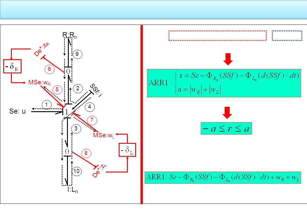
263
OUR DC MOTOR

264
Robust ARR From BG DC motor
Uncertain ARRs R(t) adaptive thresholds (t)
 adaptive thresholds. (t)")
265
Residuals in normal operation
Simulation results Residuals in normal operation

266
Simulation results Réaction des deux résidus robustes suite à une variation des paramètres RA et RM d'une valeur supérieure à leur incertitude relative

267
Simulation results Réaction des deux résidus robustes suite à une variation des paramètres RA et RM d'une valeur égale à leur incertitude relative

268
Fault detectability index DI
The fault detectability index DI is the difference in absolute value between the effort (or flow) provided by faults and those granted by all the uncertainties.
 provided by faults and those granted by all the uncertainties.")
269
CONCLUSIONS The interest of the presented approach :
consists in the use of only one representation (bond graph modelling) for ARRs and dynamics models generation in symbolic format. the industrial designer can easily (because of integration of the functional tool as interface with the human operator) build the thermofluid dynamic model and ARRs Propose to the user a sensor placement to satisfy a given technical specification To add a new component in the data base in a generic way What are the limits in model based supervision ? The performances depend on the accuracy of the model Processes are no stationary : the models change There is not “the” method for supervision… but integration of tools is needed Real time applications are not yet used in industry : maintenance of implemented algorithms is difficult.
 for ARRs and dynamics models generation in symbolic format. the industrial designer can easily (because of integration of the functional tool as interface with the human operator) build the thermofluid dynamic model and ARRs. Propose to the user a sensor placement to satisfy a given technical specification. To add a new component in the data base in a generic way. What are the limits in model based supervision The performances depend on the accuracy of the model. Processes are no stationary : the models change. There is not the method for supervision… but integration of tools is needed. Real time applications are not yet used in industry : maintenance of implemented algorithms is difficult.")
270
APPLICATION to A steam generator Installation

271
Steps of performing a supervisory system
Failure Modes Analysis, Effects and Criticality Analysis,(AMDEC) Sensor Placement Ofline List of pertinent equipments Offline monitorability and reconfigurability analysis conditions Results of monitorability and reconfigurability analysis Elaboration of the supervision system Algorithms Online test of the supervision system Online
 Sensor Placement. Ofline. List of pertinent equipments. Offline monitorability and reconfigurability analysis conditions. Results of monitorability and reconfigurability analysis. Elaboration of the supervision system. Algorithms. Online test of the supervision system. Online.")
272
Different steps for on line diagnosis system design
Measurements for monitoring Sensors Decision making tool for supervision (FDI and FTC levels) Dynamic model List of faulty components Model Validation Logic decision procedures Ofline diagnosability analysis Measurements for FDI and control Isolation decision procedure Diagnosis algorithms generation ARRs On line FDI
 Dynamic model. List of faulty components. Model Validation. Logic decision procedures. Ofline diagnosability analysis. Measurements for FDI and control. Isolation decision procedure. Diagnosis algorithms generation. ARRs. On line FDI.")
273
Steam generator : P &IDiagram
CONDENSER HEAT-EXCHANGER V8 Condensate V4 V5 LG 2 LC Aero-refrigerator TIR 26 Environment FIR 23 24 27 21 Cooling water P3 P4 22 TC 5 PR 20 LIR 19 18 V3 25 Process delay system FIR 10 PR 11 PIR 16 TR 17 PC 2 14 15 38 29 31 V1 V6 User 13 12 ZC 1 V2 V11 STEAM FLOW FIR 3 P2 P1 V9 STORAGE TANK TIR 2 LIR 1 LG LIR 9 8 LG 1 TR 5 PC PIR 7 6 Q 4 Thermal resistor LC V10 60kW BOILER FEED WATER

274
General views Data acquisition system GUI

276
Architecture of the supervisions system

277
General Informations Number of sensors 28 Number of actuators 8
10 Pressure sensors, 12 Temperature sensors, 5 Level sensors, 4 Flow sensors, 1 Power sensor Number of actuators 8 1 Pump (switching level control in the boiler) 1 Thermal resistor (switching pressure control in the boiler) 1 Valve (Continuous pressure control in the condenser) 1 Valve (Continuous valve position) 3 discharge valves (switching level control in the condenser) 1 Three way-valve (continuous cooling water temperature control ) Number of equipment units 1 storage tank of 0.4 m3 , 4 Pumps, 1 Boiler of m3 , 5 controlled valves, 1 Controlled three-way-valve 1 Condenser coupled with an exchanger, 1 Aero-refrigerator, 1 Thermal resistor of 60 KW, 1 PC-based digital control system, 1 process delay system Automation System: Conventional instrumentation The used technology is the 4-20 mA Control system Two types of digital controllers are used: « On-off » and PI Controlled parameters: Boiler pressure, boiler level, condenser level, condenser pressure, Steam flow valve position and Cooling water temperature.
 1 Thermal resistor (switching pressure control in the boiler) 1 Valve (Continuous pressure control in the condenser) 1 Valve (Continuous valve position) 3 discharge valves (switching level control in the condenser) 1 Three way-valve (continuous cooling water temperature control ) Number of equipment units. 1 storage tank of 0.4 m3 , 4 Pumps, 1 Boiler of m3 , 5 controlled valves, 1 Controlled three-way-valve. 1 Condenser coupled with an exchanger, 1 Aero-refrigerator, 1 Thermal resistor of 60 KW, 1 PC-based digital control system, 1 process delay system. Automation System: Conventional instrumentation. The used technology is the 4-20 mA. Control system. Two types of digital controllers are used: « On-off » and PI. Controlled parameters: Boiler pressure, boiler level, condenser level, condenser pressure, Steam flow valve position and Cooling water temperature.")
278
General Informations Failure scenarios Reconfigurability Plant faults
Water leak in the boiler by opening valve V11 Thermal insulation fault taking off the calorifuge sheet Pressure leak in the steam flow system by opening valve V3 Water leak in the storage tank by opening valve V10 Steam pipe blocked out by closing the manual valve V13 Actuator faults Any valve can be blocked open or closed Pump fault by switching off the power supply The actuator control signals can be modified Failure Discharge valves leak by opening valve V8 et V9 Sensor abrupt faults Any sensor can be temporary disconnected The sensor signals can be modified Reconfigurability Degraded mode: one or two discharge valves in running Use of one or two controlled valves in the steam flow system The long loop of the heat-exchanger in fault mode: degraded mode, only the short loop is in running mode Feeding pumps are redundant Sensor system can be reconfigured

279
Modelling hypothesis For the feeding circuit the liquid is incompressible. I n the steam boiler, water and steam are in thermodynamic equilibrium, This is justified by the fact that we have a good homogenous mixture of the emulsion water-steam. The mixture is at uniform pressure, which means that we neglect surface tension of the steam bubbles. The boiler has a thermal capacity and is subject to heat losses towards the environment All variables are described by lumped parameters.

280
WORD BOND GRAPH OF THE INSTALLATION
Voltage source i U Thermal resistor Condenser Cooling circuit Condenser-Heat exchanger Boiler Steam expansion Discharge valves Feed water circuit Receiver

281
Bond graph model

282
Dynamic simulation using Bond graph and Matlab Simulink

283
Modular Approach using library models

284
Model Validation Real system Sensors (Acquisition card) + - No
yr(t) u(t) + Model - ym(t) No < adm? yes Validated model
 u(t) + Model. - ym(t) No. < adm yes. Validated model.")
285
ARRs generation

287
Diagnosability analysis : Fault Signature matrix
23 RRAs générées Modèle bond graph sous forme icone métier Bibliothèque de modèles Matrice de surveillabilité

288
Control algorithm based on Panorama software

289
Variable definition based on Panorama software

290
Diagnosis Decision procedure based on Panorama software

291
Diagnosis Decision procedures based on Panorama software

292
Determination of thresholds

293
CONCLUSIONS The interest of the presented approach :
consists in the use of only one representation (bond graph modelling) for ARRs and dynamics models generation in symbolic format. the industrial designer can easily (because of integration of the functional tool as interface with the human operator) build the thermofluid dynamic model and ARRs Propose to the user a sensor placement to satisfy a given technical specification To add a new component in the data base in a generic way What are the limits in model based supervision ? The performances depend on the accuracy of the model Processes are no stationary : the models change There is not “the” method for supervision… but integration of tools is needed Real time applications are not yet used in industry : maintenance of implemented algorithms is difficult.
 for ARRs and dynamics models generation in symbolic format. the industrial designer can easily (because of integration of the functional tool as interface with the human operator) build the thermofluid dynamic model and ARRs. Propose to the user a sensor placement to satisfy a given technical specification. To add a new component in the data base in a generic way. What are the limits in model based supervision The performances depend on the accuracy of the model. Processes are no stationary : the models change. There is not the method for supervision… but integration of tools is needed. Real time applications are not yet used in industry : maintenance of implemented algorithms is difficult.")
Similar presentations


 By Hariharan Kannan.>")


