1. Electrochemistry for Engineers
Electrochemistry for Engineers
LECTURE 3
Lecturer: Dr. Brian Rosen
Office: 128 Wolfson
Office Hours: Sun 16:00

2. What Have We Done So Far?? Thermodynamics of electrode potentials
Use of 2 electrodes connected in Galvanic and Electrolytic configurations
Effect of kinetic parameters on electrode polarization (I-V) relationships
Effect of exchange current density
Effect of barrier symmetry

3. Polarization under Activation Control
jac

4. Mixed Control

5. Mass Transport at Electrodes

6. General Statement of Mass Transport to a Planar Electrode
Mass transfer to an electrode is governed by the Nernst-Planck equation. For one-dimensional mass transfer of a species i (or j) along the x-axis:
where Ji is the flux of species i(mol sec-1 cm-2) at a distance x from the surface.
Di is the diffusion coefficient (cm2/sec)
is the concentration gradient at a distance x,
is the potential gradient
zi and Ci are the charge and concentration of species i, respectively,
v(x) is the velocity (cm/sec) with which a volume element in solution moves along the axis.

7. Meaning of Terms
• 1st term: diffusion. Movement of a species under the influence of a gradient of chemical potential (i.e., a concentration gradient).
• 2nd term: migration. Movement of a charged body under the influence of an electric field (a gradient of potential).
• 3rd term: convection. Stirring or hydrodynamic transport, but also natural convection (convection caused by density gradients) and forced convection.

8. 1st Fick’s law: How does diffusion change the concentration profile
with respect to space
where: DO is a diffusion coefficient of the species “O”, in cm2/s, usually ca cm2/sec.
We are seeking a current vs. time relationship!

9. 2nd Fick’s law: How does diffusion affect the concentration grad with respect to time?
Is controlled by mass transport only!
This yields the diffusion-limited current id
All lead to a definition of chronoamperometry, measurements of currents vs. time, under potential step conditions.
Under the boundary conditions:
The initial condition = the homogeneity condition (before the experiment starts at t = 0):
The semi-finite condition (regions sufficiently distant from the electrode are unperturbed by the experiment):
The surface condition after the potential transition:

10. Forms of the Laplacian Operator for Different Geometries
Generalizing for Any Geometry
Where is the Laplacian operator
Forms of the Laplacian Operator for Different Geometries
Type
Linear
Rectangular
Spherical
Cylindrical (axial)
Variables x
x,y,z r
Laplacian
Example
Planar disk electrode
Cube-shaped electrode
Hanging drop electrode
Wire (rod) electrode

11. The Cottrell Experiment
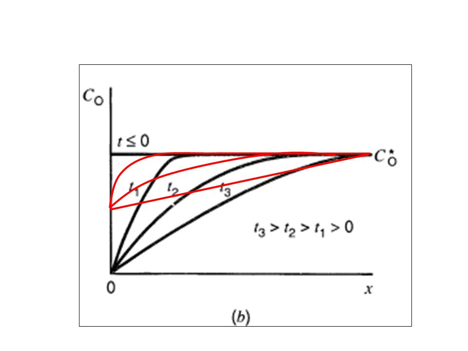
A: surface area in cm2; n, a number of electrons per molecule (ion), dimensionless;
F, the Faraday constant.
(The flux equation gives the current in Amperes.)
Flux, and electric current, may be entirely controlled by mass transport of the species “O” to the electrode surface.
A potential step experiment:
Only “O” is initially present
t <0, E = E1, no reaction initiation (well above EO)
t ≥0, E = E2, reaction occurs
E2 is sufficiently negative (in case of reduction) that C(0,t)=0
A reversible reaction: O+ne R

12. Boundary Conditions for Cottrell Experiment
The initial condition
CO(x,t) = CO* for t<0
The semi-finite condition (regions sufficiently distant from the electrode are unperturbed by the experiment):
The surface condition after the potential transition:
CO(0,t) = 0 for t<0
t > 0

13. Laplace Transformation
The Laplace transform in t of the function F(t) is symbolized by L{F(t)}, f(s), or and is defined by: ∞
The existence of the transform is conditional:
F(t) must be bound at all interior points on the interval 0 ≥ t < ∞;
that it has an infinite number of discontinuities; and
that is to be of an exponential order
In practical applications, (a) and (c) do occasionally offer obstacles, but (b) rarely does.

14. The Laplace transformation is linear in that:
The Table gives a short list of commonly encountered functions and their transforms (p. 771).
The Laplace transformation is linear in that:
Table: Laplace Transforms of Common Functions
F(t)
A(constant)
e-at
sin at
cos at
sinh at
cosh at t
t(n-1)/(n-1)!
(t)-1/2
2(t/)1/2
erfc[x/2(kt)1/2]
exp(a2t) erfc(at1/2)
f(s)
A/s
1/(s+a)
a/(s2+ a2)
s/(s2 + a2)
a/(s2 - a2)
s/(s2 - a2)
1/s2
1/sn
1/s1/2
1/s3/2
e-x, where  = (s/k)1/2
e-x /
e-x /s
e-x /s 

15. Solutions of Partial Differential Equations
There is a need for solving the diffusion equation (PDE):
The solution requires an initial condition (t = 0), and two boundary conditions in x. Typically one takes C (x, 0) = C* for the initial state, and the semi-infinite condition:
“This requires only one additional boundary condition to define a problem completely.” Without, a partial solution can be obtained.
for t > 0

16. Solutions of Partial Differential Equations (whiteboard)

17. Transforming (Laplace) the PDE on the variable t, we obtain
We then obtain (ODE):
and, after transformation of the semi-infinite condition
hence, B’(s) must be zero for the second boundary condition.

18. Then to solve, we must take the reverse transform:
Final evaluation of
depends on the third boundary condition.
and

19. Application of Laplace transformation and the first 2 boundary conditions
to the 2nd Fick’s equation yields (see above):
Using the surface condition, the function A(s) can be evaluated, and:
can be inverted to obtain the concentration profile for species O.
Transforming the surface condition gives (evaluate A’(s)):
Which implies that: A=-Co*/s
Inversion using inverse Laplace transform gives the concentration profile,
to be developed!

20. Concentration Profile Solution

21. Obtaining Current vs. Time
The flux at the electrode surface is proportional to current:
Which is transformed to:

22. The Cottrell equation for a reversible Faradaic reaction!
Substitution of yields (at x = 0):
and inversion produces the current-time response:
The Cottrell equation for a reversible Faradaic reaction!
The Cottrell equation predicts:
an inverted t1/2 current-time relationship
at t approaching zero the current goes to infinity
current measured is always proportional to the bulk concentration of “Ox”.
A planar electrode! R is initially absent!

23. Qualitative Understanding of Cottrell Experiment
Concentration Grad
CO(x,t) vs. x
Potential Pulse
E vs. t
Current Response
i vs. t

24. Sampled Current Voltammetry
Cottrell Experiment only valid for point 5
Cottrell equation is only valid if we assume the overpotential ,E-E°, was
negative enough to keep our boundary condition CO (0,t)=0
Only at large overpotentials can we assume that the surface
concentration will be zero because of the large rate of reaction!
When the surface concentration is zero, the current is limited only by diffusion
This is the “diffusion limiting current”, id

25. DO NOT CONFUSE
“Fast kinetics” – Electron transfer is rapid, therefore surface
concentration of O and R can be assumed to obey the Nernst equation
“Fast Rate of Reaction” – Reaction occurs quickly due to large driving force a high overpotentials. Therefore, the surface concentration of
reactant can be assumed as zero.
For example, in a reduction reaction one can have fast kinetics at but a low rate of reaction because the potential is just below E0

26. NEW Boundary condition
Generalized Case (points 1,2,3, or 4)
for a step of any size
Fast kinetics, therefore CO(0,t) and CR(0,t) obey the Nernst Equation
Initial condition
Semi-infinite
NEW Boundary condition
(requires knowing
CR (0,t) since
boundary condition
of Cottrell does not
apply)
…since a gain in R is a loss in O according to O + ne  R

27. Laplace transformation of Ficks second law on “O” and “R” in
consideration of initial and semi-infinite conditions gives:
Application of the new boundary condition shows that B(s) = -A(s)ξ
Where ξ = , the root-ratio of the diffusion coefficients of the
reduced ‘R’ and oxidized ‘O’ species

28. …upon reverse transformation, we get:
The difference between the GENERALIZED expression and the COTTRELL expression
(at large overpotentials) is a factor of 1/(1+ξϴ)

29. in their standard concentrations! The reduction of O still occurs
Important!!!
Why does cathodic current flow above E0?
Recall: At E0, the oxidation and reduction reaction rates are equal assuming O and R are present
in their standard concentrations! The reduction of O still occurs
ABOVE E0 but the oxidation of R occurs faster giving a net anodic current.
Here, a net cathodic current is seen, even above E0, since R does not exist initially

31. Reversibility

32. Double Potential Step

33. but…. Therefore, experimentally measured current includes
the interface of the electrode and the electrolyte form a capacitor!
Therefore, experimentally measured current includes
non-electrochemical (non-Faradaic) currents!!!

34. The Electrical Double Layer

35. Review: RC Circuits
When a capacitor is charged in a circuit, it acquires a potential difference between the plates.
A typical RC circuit:
Schg is on at t = 0, the charge on the capacitor is time dependent:
q(t)chg = Qo (1- e-t/RC ) = Qo(1 - e-t/) ..where (Qo = EC)

36. The Time Constant, 
A RC circuit for charging a capacitor in a single “charge” step: The charge - time profile: q(t) = Qo(1-e-t/RC), at R =10 , C = 20 F, Q0 = 1 mC, E = 50 V

37. q(t)dis = Qo e-t/RC = Qo e-t/
At t = , the capacitor is charged to 0.63 (63%) of its final value
(Qo), q(t)  =  Qo (1-e-1)  =  0.63Qo.
At a time equal to 3, the capacitor is charged to 95% of Qo.
Upon charging to the voltage E after the switch (Schg) is on, the current in the resistor R decreases, and eventually stops.
When the capacitor is discharged, the current in the resistors starts at E/R and then decreases to zero:
q(t)dis
= Qo e-t/RC
= Qo e-t/

38. At , the charge on the capacitor is reduced to 0
At , the charge on the capacitor is reduced to 0.37 of the initial value; the discharging curve: q(t) = Qoe-t/RC:
For charging (back to):

39. i (total) = i (faradaic) + i (non-Faradaic)
= E/R.e-t/RC a b
(a) charge vs. time, and (b) current in time. Circuit parameters are: R =10 , C= 20 F. [Q0 = 20 C,  = 10  x 20 F = 0.2 ms].
i (total) = i (faradaic) + i (non-Faradaic)
From Cottrell
From DL charging
Therefore, in a POTENTIAL STEP EXPERIMENT

40. i (total) = i (faradaic) + i (non-Faradaic)
From Cottrell
From DL charging
Therefore, in a POTENTIAL STEP EXPERIMENT
= E/R.e-t/RC
Since the non-faradaic current contributes to our
experimental signal, we must figure out how to model C,
the capacitance, of an electrochemical system!
To do this, we must be able to model the interface!
Which model should we use?

41. I. The Helmholtz Model Charge density in units of charge/area
• electric charge resides on a surface of an electronic conductor, e.g. metal (in an electrochemical cell)
• The Helmholtz model: a counterion resides at the surface
2 sheets of charge densities () of opposite sign, separated by a distance of molecular order
• gives the “double layer” (dl)
Charge density in
units of charge/area
 is the stored charge density,  is the dielectric constant of the medium, 0 is permittivity of the free space, V is the voltage drop between the plates.

42. The Helmholtz Model
VISUALIZED
METAL
(M)
SOLUTION
(S)

43. Helmholtz Model - Problems
predictions (incorrect): no bulk concentration dependence of Cd:
The differential capacity (at constant parameters):

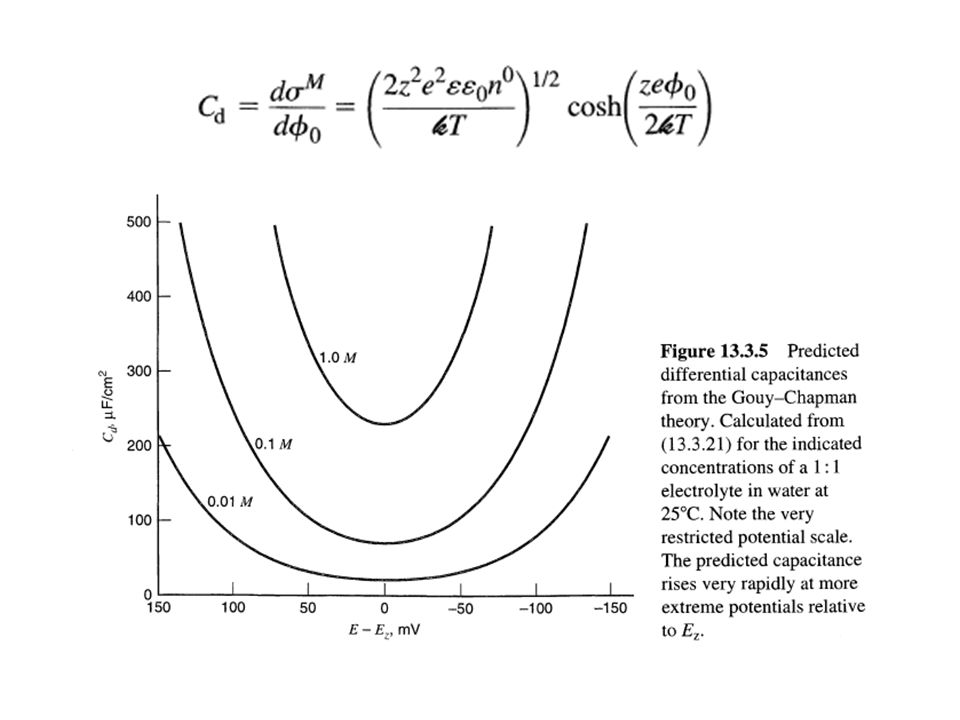
44. II. Gouy and Chapman
Interplay of two tendencies at the metal solution interface:
- the tendency of the electrostatic interactions between ions and the charged plane
- the tendency of thermal motions
The result:
• the idea of a diffuse layer
• used a statistical mechanical approach to the diffuse dl description
The model did much better (than the Helmholtz (H) model) but did not yield a satisfactory description of real system

45. Components of the G-C theory
• a solution sub-divided into laminae, parallel to the electrode and of thickness dx,
• all laminae are in thermal equilibrium with each other
• ions of any species i are not at the same energy in the various laminae, because the electrostatic potential f varies

46. Hence:
• the number concentrations of species in two laminae has a ratio determined by a Boltzmann factor
• take a reference lamina far from the electrode, where every ion is at its bulk concentration ni0
• then the population in any other lamina is:

47. II. Gouy and Chapman VISUALIZED
METAL
(M)
SOLUTION
(S)

48. f is the potential at a given point with respect to the bulk solution, e is the electronic charge, k is the Boltzmann constant, T is the absolute temperature T, and the zi is the ion charge.
The total charge per unit volume in any lamina is then:
i runs over all ionic species. r(x) is related to the potential at distance x by the Poisson equation:
By combining these equations, one obtains the Poisson-Boltzmann equation:
Substituting the property:

49. gives: Separate and integrate: gives: far from electrode the field=
Separate and
integrate:
gives:
far from
electrode
the field
is zero , ,

50. Half angle relation:
Hyperbolic cosine:
Symmetric electrolytes, ni0 (anions) = ni0 (cations) = n0, the number concentration of each ions:
“2:2”, “1:1”, z:z
Substituting: , and using the number concentration of each ion in the bulk, n0.
Anions Cations

51. A square root, both sides:
: the electric field or the field strength; the gradient of potential at a distance x.

52. = 0e-x After separating d and dx and integrating over  0 and 0x
Where  is a constant at constant T; For dilute aqueous solutions at 25 °C, ɛɛ0 = 78.4, Boltzman K is x J/K:
 = (3.29 x 107)zC*1/2
where C is in mol/L and  is in cm-1.
At small 0 (<50/z mV at 25 °C):
= 0e-x
1/: the characteristic thickness of the diffuse double layer

53. = 0e-x 1/: the characteristic thickness of the diffuse double layer
At small 0 (<50/z mV at 25 °C):
= 0e-x
1/: the characteristic thickness of the diffuse double layer

54. One More Step! How to get Capacitance?
Electric field = = 0 for all surfaces
Except the electrode itself. On the surface
= (dɸ/dx) at x=0
(notes to be posted)

55. Recall from earlier:

57. Still not completely correct
Guoy Chapman
Real Systems

58. III. The Stern Model
Stern combined the H and G-C theory and offered the most complete model for electrical dl without surface phenomena: chemisorption (specific adsorption), surface oxidation, reconstruction, relaxation, phase transitions, etc..

59. The inner layer: the compact Helmholtz or Stern layer; the inner Helmholtz plane (IHP), at the distance x1. Specifically adsorbed ions.
Solvated ions can approach the metal at the distance x2 (the locus of the center of such non specifically adsorbed ions is called OHP).