1. Eigenmode Expansion Methods for
Simulation of Silicon Photonics - Pros and Cons
Dominic F.G. Gallagher
Thomas P. Felici

2. EME = “Eigenmode Expansion”
Outline
EME = “Eigenmode Expansion”
Introduction to the EME method
- basic theory
- stepped structures
- smoothly varying
- periodic
Why use EME?
Comparison to BPM and FDTD
Examples

3. A B
modes:
“The fields at AB of any solution of Maxwell’s Equations may be written as a superposition of the modes of cross-section AB”.

4. Basic Theory propagation constant electric field magnetic field
forward amplitude
backward amplitude
mode profiles
exact solution of Maxwell’s Equations
bi-directional

5. so far only z-invariant what about a step change?
am(+)
bm(+)
bm(-)
am(-)
Maxwell's Equations gives us continuity conditions for the fields, e.g. the tangential electric fields must be equal on each side of the interface

6. Applying continuity relationships, eg:
LHS
forward
backward
forward
backward
RHS
With orthogonality relationships and a little maths we get an expression of the form:
SJ is the scattering matrix of the joint

7. Straight Waveguide A B
trivial - the scattering matrix is diagonal:

8. Example: S-matrix decomposition of an MMI couplerB C D E

9. Evaluating S-matrix of deviceB C D E AB C DE
ABC DE
ABCDE

10. Smoothly Varying Elements
Problem: modes are changing continuously along element
Thus each cross-section requires a large computational effort to locate the set of modes
This was the major hurdle that has in the past restricted application of EME
FIMMPROP (our implementation of EME) has tackled these problems, enabling EME to be used realistically for the first time even for 3D tapering structures.

11. 0 Order (Staircase Approximation)hn hn
Set of local modes computed at discrete positions along taper
Simple to implement
theoretically accurate as Nsliceà ¥
errors grow as Nsliceà ¥ so practical limit on Nslice
can get spurious resonances between modes for long structures and small Nslice

12. 1st Order (Linear Approximation)hn
analytic integration hn
Set of local modes computed at
discrete positions along taper
More complex to implement
good accuracy for modest Nslice
errors à 0 for modest Nslice
need only small number of modes

13. Showing zero order versus first order result

14. Periodic Structures A B A B A B A B A B P1 P1 P1 P1 P1 P2 P2 P3 S
compute time µ log(Nperiod)
i.e. almost as quick as a straight waveguide! S

15. Bends transmission = (Sj)N Sj periodic structure
bend is just periodic repeat of straight waveguide sections!

16. Boundary Conditions
PEC & PMC (perfect electric/magnetic conductors) - useful for exploiting symmetries
transparent boundary conditions
PML’s - perfect matched layers (with PEC or PMC)
Transparent BC’s are naturally formed at input and output of EME computation
finding eigenmodes with true transparent boundary conditions leads to leaky modes - leaky modes cause problems with completeness of basis set.
PML much better suited for finding modes for EME than leaky modes - completeness better achieved.

17. The Perfect Matched Layer (PML)
d1 (real)
d2=a+jb
PEC
PEC
waveguide core/cladding
PML
Imaginary thickness of PML absorbs light propagating towards boundary
as much absorption as we wish with no reflection at cladding/PML interface!
guided modes not absorbed at all - nice!

18. Effect of PML on guided and radiating modes
guided mode
unbound mode
PML
core

19. PML’s with segmented waveguide

20. Why Use EME? EME Advantages
1. rigorous solution of Maxwell's Equations
- rigorous as Nmode ® infinity
- large delta-n

21. EME Advantages EME Advantages 2. inherently bi-directional.
- unconditionally stable since always express (outputs) = S.(inputs)
- takes any number of reflections into account
- not iterative
- even highly resonant cavities
- mirror coatings, multi-layer

22. Input 1 ® calculate ® Result 1 Input 2 ® calculate ® Result 2
EME Advantages
3. The S-matrix technique provides the solution for all inputs!
- component-like framework where the S-matrix of one component may be re-used in many different contexts.
Other methods:
Input 1 ® calculate ® Result 1
Input 2 ® calculate ® Result 2
Input 3 ® calculate ® Result 3
EME/FIMMPROP:
Calculate S matrix
Input 1 ® Result 1
Input 2 ® Result 2
Input 3 ® Result 3

23. EME Advantages
4. Hierarchical algorithm permits re-use, accelerating computation of sets of similar structures. When one part of a device is altered only the S-matrix of that part needs to be re-computed.
Initial evaluation time: ~ 2:54 m:s
change period - time: ……
change offset - time: ….

24. Design Curve Generation
Traditional Tool:
5 mins
5 mins
5 mins
5 mins
5 mins
5 mins
EME/FIMMPROP:
5 mins
3 mins

25. EME Advantages 5. Wide-angle capability
- wider angle - just add more modes - adapts to problem

26. EME Advantages very thin layers - wide range of dimensions
6. The optical resolution and the structure resolution may be different.
- c.f. BPM (stability problems with non-uniform grid)
very thin layers - wide range of dimensions
no problem for EME/FIMMPROP algorithm does not need to discretise the structure

27. Right: plasmon between silver plates
Plasmonics
Right: plasmon between silver plates
EME is a rigorous Maxwell solution and can model many plasmonic devices (provided basis set is not too large).

28. Why Use EME? Disadvantages
Structures with very large cross-section are less suitable for the method since computational time typically scales in a cubic fashion with e.g. cross-section width.
The algorithms are much more complex to write - for example it is very difficult to ensure that a mode has not been missed from the basis set.
EME is not a "black box" technique - the operator must make some effort to understand the method to use it to his best advantage.

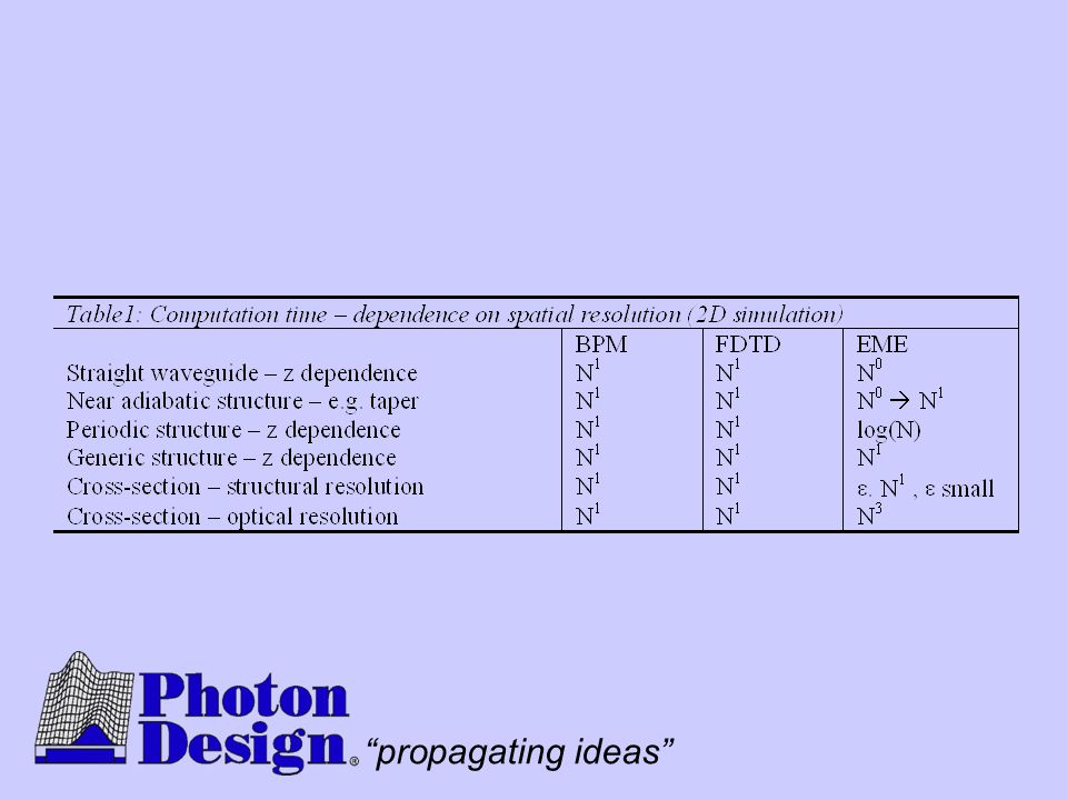
29. Computation Time Compare computation time with BPM and FDTD
Restrict our discussion to 2D - i.e. z and one lateral dimension
Both BPM and FDTD require a finite difference grid sampling the structure, this same grid used for optical field
EME does not need a structure grid (FMM Solver)
Equivalent of grid in EME is the number of modes
For straight wg, EME particularly efficient
Periodic section - logarithmic time
Arbitrary z-variations - all 3 methods have similar dependence with z-complexity/resolution
In lateral dimension EME gets high spatial resolution almost for free. (c.f. BPM, non-uniform grid problems…)
But lateral optical resolution - compute time µ N3
the limiting factor in EME

31. Memory Requirements
Very efficient as a function of z-resolution - N0 scaling for straight or periodic

32. Applications
We present a variety of examples illustrating EME features

33. SOI Waveguide Modes
Ex Field
Ey field

34. The MMI MMI ideal for EME - inherently a modal phenomenon 8 modes
Illustrate design scan simulations for price of two!

35. Tapered Fibre
6 modes
“how long for 98% efficiency?” - ideal question for EME

36. 50 simulations in scan 6.5s per simulation (in 3D!) 1 0.9 0.8 0.7 0.6
taper efficiency
0.5
0.4
0.3
0.2
0.1
2000
4000
6000
8000
10000
taper length (mm)
50 simulations in scan
6.5s per simulation (in 3D!)

37. Effective indices of first 5 modes
1.472
1.470
1.468
1.466
1.464
Mode eff. index
1.462
1.460
1.458
1.456 10 20 30 40 50 60 70 80 90
100
z-position (um)
Strong coupling occurs when the effective indices are close - telling us where the trouble spots of the device are.
Powerful diagnostic - tells designer where to improve the design

38. Co-directional Coupler
remember logarithmic with N periods
very thin layer - no problem

39. propagation at sub-wavelength scales, including metal features

40. Ring Resonator Nmodes = 60 (for one ring)
Nmodes much higher here - wide angle propagation.
BPM gives nonsense

41. Photonic Crystal Design
Nmodes = 60 (for one ring)
Nmodes much higher here - wide angle propagation.
BPM gives nonsense

42. VCSEL Modelling Rtop Rbot Resonance Condition top DBR mirror
active layer
lower DBR mirror
Rtop
Rbot

43. Showing the domains of applicability of FDTD, BPM and EME to varying delta-n and device length.

44. Showing the domains of applicability of FDTD, BPM and EME to varying numerical apperture and cross-section size.

45. BPM – Capability Scores
Aspect
Performance
Score/10
Speed
FD-BPM scales linearly with area and can take fairly long steps in propagation direction -
Memory
Usage scales linearly with c/s area NA
Best with low NA simulations. Versions using Pade approximants can model a beam travelling at a large angle but still cannot deal well with light simultaneously travelling at a wide range of angles. 4
Delta-n
Best with low delta-n simulations. 5
Polarisation
Semi-vectorial versions work best. Still problems modelling mixed or rotating polarisation structures accurately
Lossy materials
Can model modest losses efficiently. Most versions cannot deal well with metals 7
Reflections
Some success in implementing reflecting/bi-directional BPM but generally avoided due to slow speed and stability problems 3
Non-linearity
FD-BPM can model non-linearity. 9
Dispersive
Being a frequency-domain algorithm this is easy 10
Geometries
The BPM grid allows diffuse structures to be modelled easily. Problems modelling non-rectangular structures accurately on the rectangular grid
ABCs
PMLs available and work well

46. FDTD – Capability Scores
Aspect
Performance
Score/10
Speed
Scales as V (device volume) but grid size is small so not as good as BPM or EME for long devices. -
Memory NA
Omni-directional algorithm is agnostic to direction of light – great when light is travelling in all directions 10
Delta-n
Rigorous Maxwell solver, happy with high delta-n, but slows down somewhat with high index. 9
Polarisation
Rigorous Maxwell Solver is polarisation agnostic
Lossy materials
Can model even metals accurately with a fine enough grid and small modifications to the algorithm.
Reflections
Yes – easy and stable even when there are many reflecting interfaces.
Non-linearity
Yes – non-linear algorithm relatively easy to do
Dispersive
Have to approximate the dispersion spectrum with one or more Lorentizans but exact fit to the spectrum over a wide wavelength is difficult and the algorithm also slows down. 7
Geometries
Fine rectangular grid can do arbitrary geometries easily, though there are problems approximating diagonal metal surfaces 8
ABCs
Yes – very effective and easy to use

47. EME – Capability Scores
Aspect
Performance
Score/10
Speed
EME scales poorly with cross-section area – as A3 (A is c/s area). However it can efficiently model very long structures especially if their cross-section changes only slowly or occasionally. Periodic structures scale as log(number of periods) – so can compute efficiently. S-matrix approach allows a set of similar simulations to be done very quickly – parts of previous calculation can be reused. -
Memory
Memory increases at rate between A2 and A3 (A is c/s area), but very efficient for long or periodic devices. NA
Can model wide-angle beams by increasing the number of modes in the basis set at expense of speed and memory. 7
Delta-n
Rigorous Maxwell Solver can accurately model high delta-n 8
Polarisation
Rigorous Maxwell Solver is polarisation agnostic 10
Lossy materials
Depends on mode solver used.
Reflections
Yes – easy and stable even when there are many reflecting interfaces.
Non-linearity
Difficult – have to iterate, and then only modest non-linearity levels will converge 3
Dispersive
Being a frequency-domain algorithm this is easy
Geometries
Depends on the mode solver used. Can use different structure discretisations in different cross-sections, so solver can better adapt to the geometry.
ABCs
Depends on the mode solver used. E.g. a finite-difference solver can be readily constructed to implement PMLs. However, PML’s are more difficult to use with EME than with BPM or FDTD.

48. Conclusions Powerful compliment to BPM and FDTD
Exceedingly efficient/fast for wide range of examples
Rigorous Maxwell solver, bi-directional, wide angle
mode data provides important insight into workings of device.