Download presentation
Presentation is loading. Please wait.

1
Binary Search Tree AVL Trees and Splay Trees
PUC-Rio Eduardo S. Laber Loana T. Nogueira

2
Binary Search Tree Is a commonly-used data structure for storing and retrieving records in main memory

3
Binary Search Tree Is a commonly-used data structure for storing and retrieving records in main memory It guarantees logarithmic cost for various operations as long as the tree is balanced

4
Binary Search Tree Is a commonly-used data structure for storing and retrieving records in main memory It guarantees logarithmic cost for various operations as long as the tree is balanced It is not surprising that many techniques that maintain balance in BSTs have received considerable attention over the years

5
Techniques: AVL Trees Splay Trees

6
How does the BST works?

7
How does the BST works? Fundamental Property: x

8
How does the BST works? Fundamental Property: x y x

9
How does the BST works? Fundamental Property: x y x x z

10
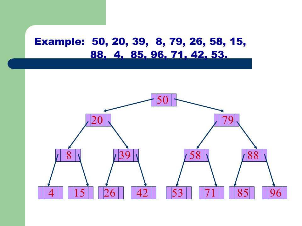
Example: 50, 20, 39, 8, 79, 26, 58, 15, 88, 4, 85, 96, 71, 42, 53. 50 20 79 8 39 58 88 4 15 26 42 53 71 85 96
11
Relation between #nodes and height of a binary tree

12
Relation between #nodes and height of a binary tree
At each level the number of nodes duplicates, such that for a binary tree with height h we have at most: h-1 = 2h – 1 nodes

13
Relation between #nodes and height of a binary tree
At each level the number of nodes duplicates, such that for a binary tree with height h we have at most: h-1 = 2h – 1 nodes Or equivalently:

14
Relation between #nodes and height of a binary tree
At each level the number of nodes duplicates, such that for a binary tree with height h we have at most: h-1 = 2h – 1 nodes Or equivalently: A binary search tree with n nodes can have mininum height h = O( log n)
")
15
BST The height of a binary tree is a limit for the time to find out a given node

16
BST The height of a binary tree is a limit for the time to find out a given node BUT...

17
It is necessary that the tree is balanced
BST The height of a binary tree is a limit for the time to find out a given node BUT... It is necessary that the tree is balanced

18
BST The height of a binary tree is a limit for the time to find out a given node BUT... It is necessary that the tree is balanced (“every” internal node has 2 children)
")
19
BST Algorithm Algorithm BST(x) If x = root then “element was found”
Else if x < root then search in the left subtree else search in the right subtree

20
Complexity of Seaching in balanced BST
O(log n)
")
21
Including a node in a BST
Add a new element in the tree at the correct position in order to keep the fundamental property.

22
Including a node in a BST
Add a new element in the tree at the correct position in order to keep the fundamental property. Algorithm Insert(x, T) If x < root then Insert (x, left tree of T) else Insert (x, right tree of T)
 If x < root then Insert (x, left tree of T) else. Insert (x, right tree of T)")
23
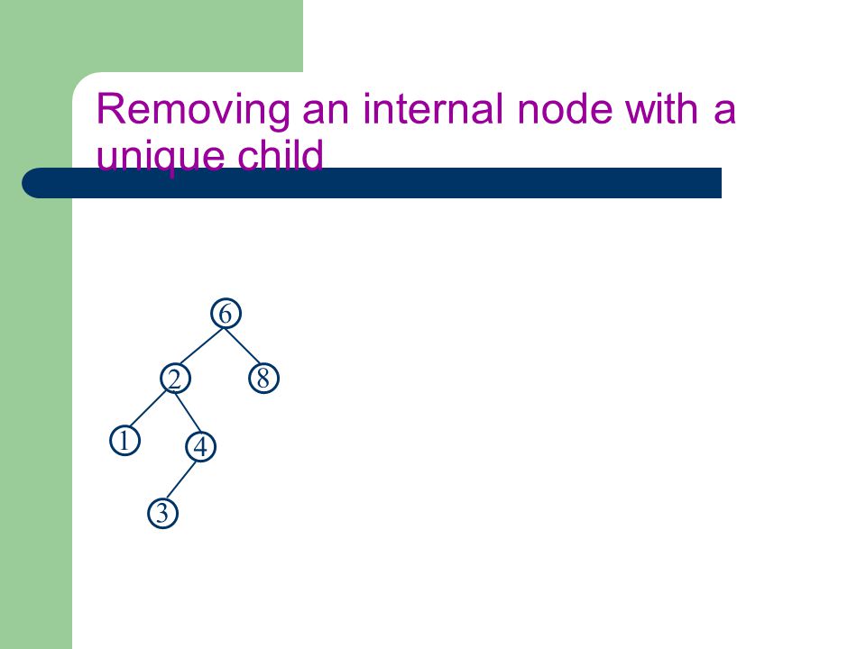
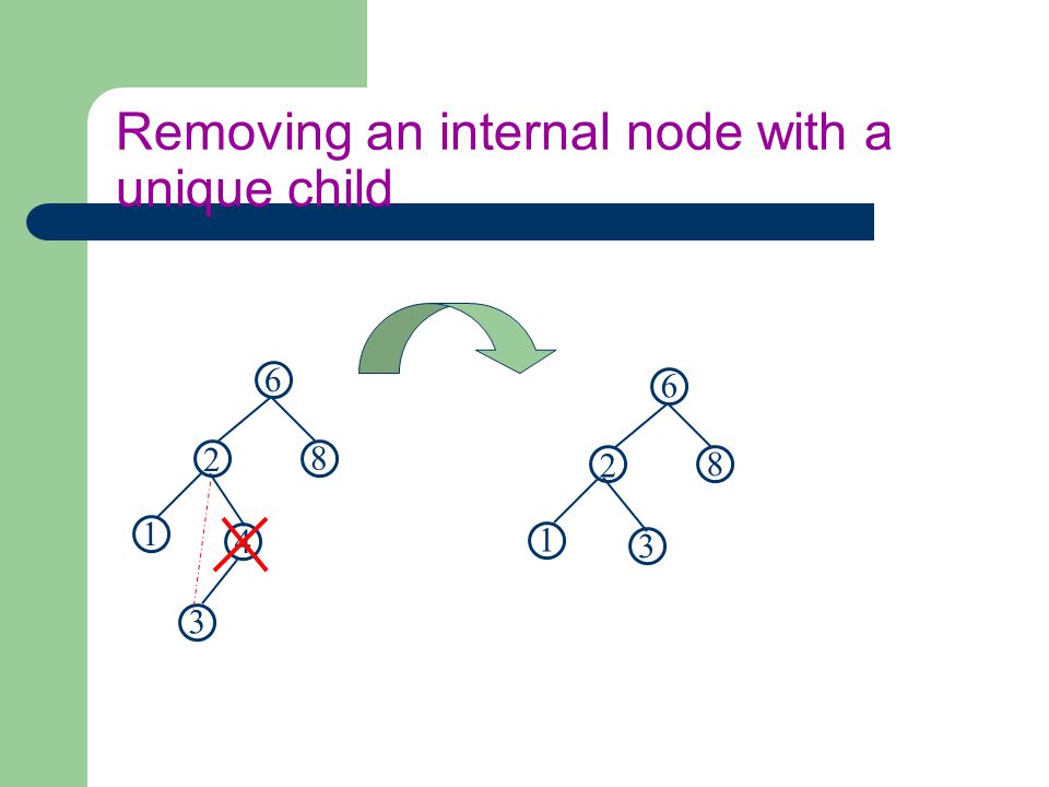
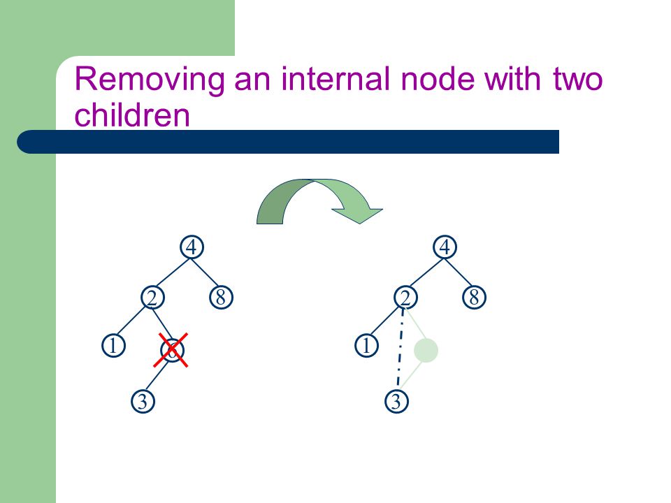
Removing a node in a BST SITUATIONS: Removing a leaf
Removing an internal node with a unique child Removing an internal node with two children

24
Removing a node in a BST SITUATIONS: Removing a leaf
Removing an internal node with a unique child Removing an internal node with two children

25
Removing a Leaf 6 2 8 1 4 3

26
Removing a Leaf 6 2 8 1 4 3

27
Removing a Leaf 6 6 2 8 2 8 1 1 4 4 3

28
Removing a node in a BST SITUATIONS: Removing a leaf
Removing an internal node with a unique child Removing an internal node with two children

29
Removing an internal node with a unique child
It is necessary to correct the pointer, “jumping” the node: the only grandchild becomes the right son.

30
Removing an internal node with a unique child
6 2 8 1 4 3
31
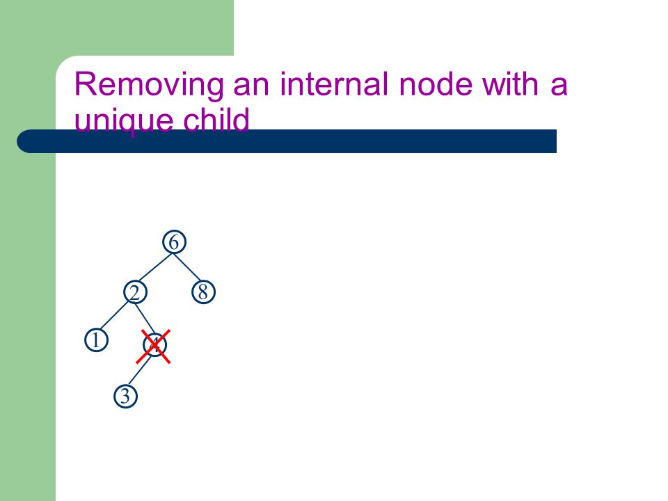
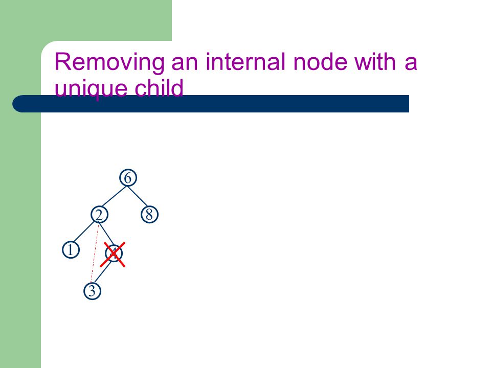
Removing an internal node with a unique child
6 2 8 1 4 3
32
Removing an internal node with a unique child
6 2 8 1 4 3
33
Removing an internal node with a unique child
6 6 2 8 2 8 1 4 1 3 3
34
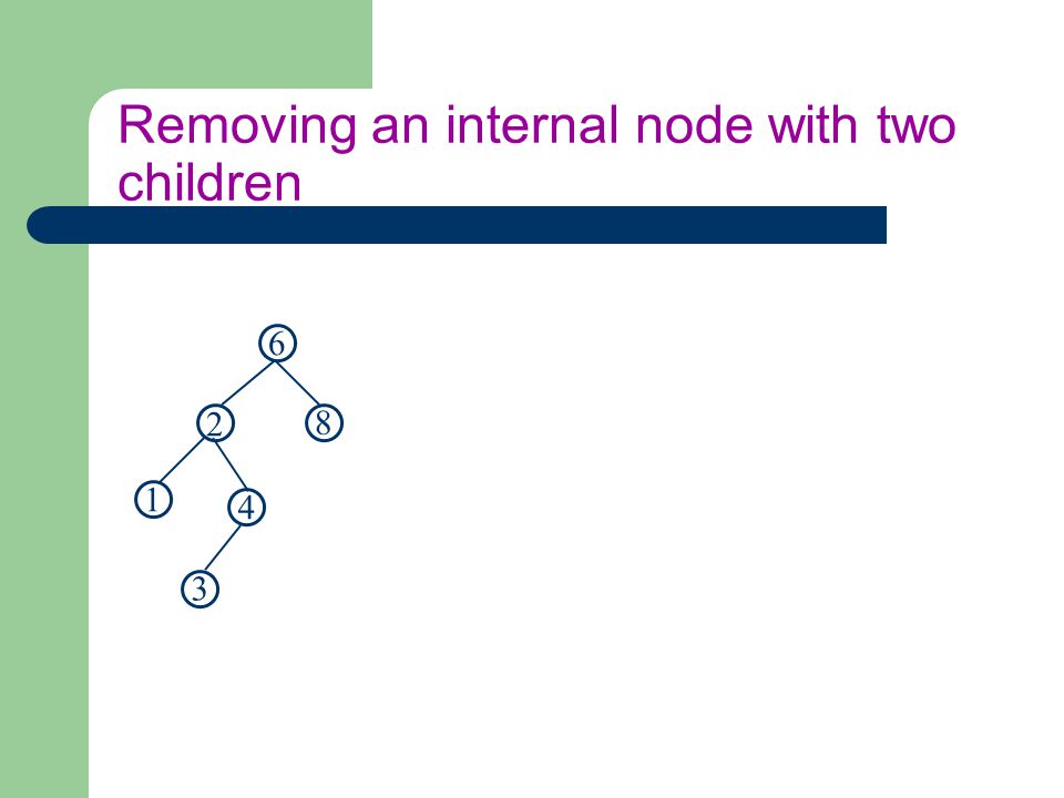
Removing a node in a BST SITUATIONS: Removing a leaf
Removing an internal node with a unique child Removing an internal node with two children

35
Removing an internal node with two children
Find the element which preceeds the element to be removed considering the ordering (this corresponds to remove the element most to the right from the left subtree)
")
36
Removing an internal node with two children
6 2 8 1 4 3
37
Removing an internal node with two children
6 2 8 1 4 3
38
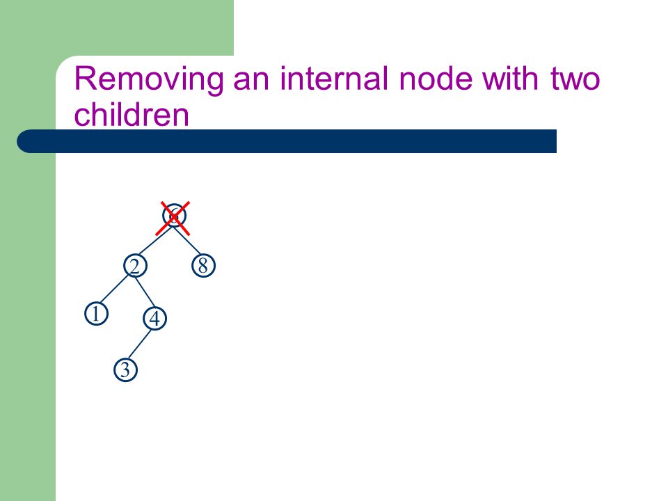
Removing an internal node with two children
6 6 2 8 2 8 1 4 1 4 3 3

39
Removing an internal node with two children
Find the element which preceeds the element to be removed considering the ordering (this corresponds to remove the element most to the right from the left subtree) Switch the information of the node to be removed with the node found
 Switch the information of the node to be removed with the node found.")
40
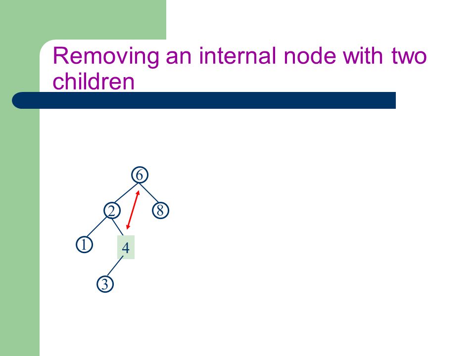
Removing an internal node with two children
6 2 8 1 4 3
41
Removing an internal node with two children
6 4 2 8 2 8 1 1 4 6 3 3

42
Removing an internal node with two children
Find the element which preceeds the element to be removed considering the ordering (this corresponds to remove the element most to the right from the left subtree) Switch the information of the node to be removed with the node found Remove the node that contains the information we want to remove
 Switch the information of the node to be removed with the node found. Remove the node that contains the information we want to remove.")
43
Removing an internal node with two children
4 2 8 1 6 3

44
Removing an internal node with two children
4 2 8 1 6 3

45
Removing an internal node with two children
4 4 2 8 2 8 1 1 6 6 3 3
46
The tree may become unbalanced

47
The tree may become unbalanced
Remove: node 8 6 2 8 1 4 3

48
The tree may become unbalanced
Remove: node 8 6 6 2 8 2 1 1 4 4 3 3

49
The tree may become unbalanced
Remove: node Remove node 1 6 6 2 8 2 1 1 4 4 3 3

50
The tree may become unbalanced
Remove: node Remove node 1 6 6 6 2 8 2 2 1 1 4 4 4 3 3 3

51
The tree may become unbalanced
The binary tree may become degenerate after operations of insertion and remotion: becoming a list, for example.

52
The tree may become unbalanced
The binary tree may become degenerate after operations of insertion and remotion: becoming a list, for example. The access time becomes no longer logarithmic HOW TO SOLVE THIS PROBLEM???

53
Balanced Trees: AVL Trees Splay Trees Treaps Skip Lists

54
Balanced Trees: AVL Trees Splay Trees Treaps Skip Lists

55
AVL TREES (Adelson-Velskii and Landis 1962)
BST trees that maintain a reasonable balanced tree all the time. Key idea: if insertion or deletion get the tree out of balance then fix it immediately All operations insert, delete,… can be done on an AVL tree with N nodes in O(log N) time (average and worst case!)
 time (average and worst case!)")
56
AVL TREES (Adelson-Velskii and Landis)
AVL Tree Property: It is a BST in which the heights of the left and right subtrees of the root differ by at most 1 and in which the right and left subtrees are also AVL trees

57
AVL TREES (Adelson-Velskii and Landis)
AVL Tree Property: It is a BST in which the heights of the left and right subtrees of the root differ by at most 1 and in which the right and left subtrees are also AVL trees Height: length of the longest path from the root to a leaf.

58
AVL TREES Example: 4 44 2 3 17 78 1 2 1 32 50 88 1 1 48 62 An example of an AVL tree where the heights are shown next to the nodes:

59
AVL TREES Example: 4 44 2 3 17 78 1 2 1 32 50 88 1 1 48 62 An example of an AVL tree where the heights are shown next to the nodes:

60
AVL TREES Example: 4 44 2 3 17 78 1 2 1 32 50 88 1 1 48 62 An example of an AVL tree where the heights are shown next to the nodes:

61
AVL TREES (Adelson-Velskii and Landis)
Example:

62
Relation between #nodes and height of na AVL tree

63
Relation between #nodes and height of na AVL tree
Let r be the root of an AVL tree of height h Let Nh denote the minimum number of nodes in an AVL tree of height h

64
Relation between #nodes and height of na AVL tree
Let r be the root of an AVL tree of height h Let Nh denote the minimum number of nodes in an AVL tree of height h T r Te Td

65
Relation between #nodes and height of na AVL tree
Let r be the root of an AVL tree of height h Let Nh denote the minimum number of nodes in an AVL tree of height h T r Te Td h-1

66
Relation between #nodes and height of na AVL tree
Let r be the root of an AVL tree of height h Let Nh denote the minimum number of nodes in an AVL tree of height h T r Te Td h-1 h-1 ou h-2

67
Relation between #nodes and height of na AVL tree
Let r be the root of an AVL tree of height h Let Nh denote the minimum number of nodes in an AVL tree of height h T r Nh ≥ 1 + Nh-1 + Nh-2 Te Td h-1 h-1 ou h-2

68
Relation between #nodes and height of na AVL tree
Nh ≥ 1 + Nh-1 + Nh-2 ≥ 2Nh-2 + 1

69
Relation between #nodes and height of na AVL tree
Nh ≥ 1 + Nh-1 + Nh-2 ≥ 2Nh-2 + 1 ≥ 2Nh-2

70
Relation between #nodes and height of na AVL tree
Nh ≥ 1 + Nh-1 + Nh-2 ≥ 2Nh-2 + 1 ≥ 2Nh-2 ≥ 2(2Nh-4)
")
71
Relation between #nodes and height of na AVL tree
Nh ≥ 1 + Nh-1 + Nh-2 ≥ 2Nh-2 + 1 ≥ 2Nh-2 ≥ 2(2Nh-4) ≥ 22(Nh-4)
 ≥ 22(Nh-4)")
72
Relation between #nodes and height of na AVL tree
Nh ≥ 1 + Nh-1 + Nh-2 ≥ 2Nh-2 + 1 ≥ 2Nh-2 ≥ 2(2Nh-4) ≥ 22(Nh-4) ≥ 22 (2 Nh-6)
 ≥ 22(Nh-4) ≥ 22 (2 Nh-6)")
73
Relation between #nodes and height of na AVL tree
Nh ≥ 1 + Nh-1 + Nh-2 ≥ 2Nh-2 + 1 ≥ 2Nh-2 ≥ 2(2Nh-4) ≥ 22(Nh-4) ≥ 22 (2 Nh-6) ≥ 23 Nh-6
 ≥ 22(Nh-4) ≥ 22 (2 Nh-6) ≥ 23 Nh-6.")
74
Relation between #nodes and height of na AVL tree
Nh ≥ 1 + Nh-1 + Nh-2 ≥ 2Nh-2 + 1 ≥ 2Nh-2 ≥ 2(2Nh-4) ≥ 22(Nh-4) ≥ 22 (2 Nh-6) ≥ 23 Nh-6 ≥ 2i Nh-2i
 ≥ 22(Nh-4) ≥ 22 (2 Nh-6) ≥ 23 Nh-6. ≥ 2i Nh-2i.")
75
Relation between #nodes and height of na AVL tree
Nh ≥ 1 + Nh-1 + Nh-2 Cases: h=1 Nh = 1 h=2 Nh = 2 ≥ 2Nh-2 + 1 ≥ 2Nh-2 ≥ 2(2Nh-4) ≥ 22(Nh-4) ≥ 22 (2 Nh-6) ≥ 23 Nh-6 ≥ 2i Nh-2i
 ≥ 22(Nh-4) ≥ 22 (2 Nh-6) ≥ 23 Nh-6. ≥ 2i Nh-2i.")
76
Relation between #nodes and height of na AVL tree
Nh ≥ 1 + Nh-1 + Nh-2 Cases: h=1 Nh = 1 h=2 Nh = 2 ≥ 2Nh-2 + 1 ≥ 2Nh-2 ≥ 2(2Nh-4) ≥ 22(Nh-4) ≥ 22 (2 Nh-6) ≥ 23 Nh-6 ≥ 2i Nh-2i Solving the base case we get: n(h) > 2 h/2-1 Thus the height of an AVL tree is O(log n)
 ≥ 22(Nh-4) ≥ 22 (2 Nh-6) ≥ 23 Nh-6. ≥ 2i Nh-2i. Solving the base case we get: n(h) > 2 h/2-1. Thus the height of an AVL tree is O(log n)")
77
Relation between #nodes and height of na AVL tree
Nh ≥ 1 + Nh-1 + Nh-2 Cases: h=1 Nh = 1 h=2 Nh = 2 ≥ 2Nh-2 + 1 ≥ 2Nh-2 ≥ 2(2Nh-4) ≥ 22(Nh-4) ≥ 22 (2 Nh-6) ≥ 23 Nh-6 ≥ 2i Nh-2i We can also get to this limit by the Fibonacci number (Nh =Nh-1 + Nh-2) Solving the base case we get: n(h) > 2 h/2-1 Thus the height of an AVL tree is O(log n)
 ≥ 22(Nh-4) ≥ 22 (2 Nh-6) ≥ 23 Nh-6. ≥ 2i Nh-2i. We can also get to this limit by the. Fibonacci number (Nh =Nh-1 + Nh-2) Solving the base case we get: n(h) > 2 h/2-1. Thus the height of an AVL tree is O(log n)")
78
Height of AVL Tree Thus, the height of the tree is O(logN)
Where N is the number of elements contained in the tree This implies that tree search operations Find(), Max(), Min() take O(logN) time.
, Max(), Min() take O(logN) time.")
79
Insertion in an AVL Tree
Insertion is as in a binary search tree (always done by expanding an external node)
")
80
Insertion in an AVL Tree
Insertion is as in a binary search tree (always done by expanding an external node) Example: 44 17 78 32 50 88 48 62
 Example:")
81
Insertion in an AVL Tree
Insertion is as in a binary search tree (always done by expanding an external node) Example: Insert node 54 44 17 78 32 50 88 48 62
 Example: Insert node")
82
Insertion in an AVL Tree
Insertion is as in a binary search tree (always done by expanding an external node) Example: Insert node 54 44 44 17 78 17 78 32 50 88 32 50 88 48 62 48 62 54
 Example: Insert node")
83
Insertion in an AVL Tree
Insertion is as in a binary search tree (always done by expanding an external node) Example: Insert node 54 44 44 4 17 78 17 78 32 50 88 32 50 88 48 62 48 62 54
 Example: Insert node")
84
Insertion in an AVL Tree
Insertion is as in a binary search tree (always done by expanding an external node) Example: Insert node 54 44 44 4 17 78 17 78 3 32 50 88 32 50 88 48 62 48 62 54
 Example: Insert node")
85
Insertion in an AVL Tree
Insertion is as in a binary search tree (always done by expanding an external node) Example: Insert node 54 44 44 4 17 78 17 78 3 32 50 88 1 32 50 88 48 62 48 62 54
 Example: Insert node")
86
Insertion in an AVL Tree
Insertion is as in a binary search tree (always done by expanding an external node) Example: Insert node 54 44 44 4 17 78 17 78 3 32 50 88 1 32 50 88 48 62 48 62 54 Unbalanced!!
 Example: Insert node Unbalanced!!")
87
Insertion in an AVL Tree
Insertion is as in a binary search tree (always done by expanding an external node) Example: Insert node 54 44 17 78 32 50 88 48 62 54 44 4 17 78 3 1 32 50 88 48 62 Unbalanced!!
 Example: Insert node Unbalanced!!")
88
How does the AVL tree work?

89
How does the AVL tree work?
After insertion and deletion we will examine the tree structure and see if any node violates the AVL tree property

90
How does the AVL tree work?
After insertion and deletion we will examine the tree structure and see if any node violates the AVL tree property If the AVL property is violated, it means the heights of left(x) and right(x) differ by exactly 2
 and right(x) differ by exactly 2.")
91
How does the AVL tree work?
After insertion and deletion we will examine the tree structure and see if any node violates the AVL tree property If the AVL property is violated, it means the heights of left(x) and right(x) differ by exactly 2 If it does violate the property we can modify the tree structure using “rotations” to restore the AVL tree property
 and right(x) differ by exactly 2. If it does violate the property we can modify the tree structure using rotations to restore the AVL tree property.")
92
Rotations Two types of rotations Single rotations Double rotations
two nodes are “rotated” Double rotations three nodes are “rotated”

93
Localizing the problem
Two principles: Imbalance will only occur on the path from the inserted node to the root (only these nodes have had their subtrees altered - local problem) Rebalancing should occur at the deepest unbalanced node (local solution too)
 Rebalancing should occur at the deepest unbalanced node (local solution too)")
94
Single Rotation (Right)
Rotate x with left child y (pay attention to the resulting sub-trees positions)
")
95
Single Rotation (Left)
Rotate x with right child y (pay attention to the resulting sub-trees positions)
")
96
Single Rotation - Example
h h+1 Tree is an AVL tree by definition.

97
Example h h+2 Tree violates the AVL definition! Perform rotation.
Node 02 added Tree violates the AVL definition! Perform rotation.

98
Example x y h h+1 h C B A Tree has this form.

99
Example – After Rotation
y x A B C Tree has this form.

100
Single Rotation Sometimes a single rotation fails to solve the problem
k2 k1 k1 k2 Z h h X h+2 X Y Y Z h+2 In such cases, we need to use a double-rotation

101
Double Rotations

102
Double Rotations

103
Double Rotation - Example
h h+1 Delete node 94 Tree is an AVL tree by definition.

104
Example h+2 h AVL tree is violated.

105
Example x y z C A B1 B2 Tree has this form.

106
After Double Rotation A B1 B2 C x y z Tree has this form

107
Insertion Part 1. Perform normal BST insertion
Part 2. Check and correct AVL properties Trace from path of inserted leaf towards the root. Check to see if heights of left(x) and right(x) height differ at most by 1
 and right(x) height differ at most by 1.")
108
Insertion If not, we know the height of x is h+3 If the height of left(x) is h+2 then If the height of left(left(x)) is h+1, we single rotate with left child (case 1) Otherwise, the height of right(left(x)) is h+1 and we double rotate with left child (case 3) Otherwise, height of right(x) is h+2 If the height of right(right(x)) is h+1, then we rotate with right child (case 2) Otherwise, the height of left(right(x)) is h+1 and we double rotate with right child (case 4) * Rotations do not have to happen at the root! Remember to make the rotated node the new child of parent(x)
) is h+1, we single rotate with left child (case 1) Otherwise, the height of right(left(x)) is h+1 and we double rotate with left child (case 3) Otherwise, height of right(x) is h+2. If the height of right(right(x)) is h+1, then we rotate with right child (case 2) Otherwise, the height of left(right(x)) is h+1 and we double rotate with right child (case 4) * Rotations do not have to happen at the root! Remember to make the rotated node the new child of parent(x)")
109
Insertion The time complexity to perform a rotation is O(1)
The time complexity to find a node that violates the AVL property is dependent on the height of the tree, which is log(N)
")
110
Deletion Perform normal BST deletion
Perform exactly the same checking as for insertion to restore the tree property

111
Summary AVL Trees Maintains a Balanced Tree
Modifies the insertion and deletion routine Performs single or double rotations to restore structure Guarantees that the height of the tree is O(logn) The guarantee directly implies that functions find(), min(), and max() will be performed in O(logn)
 The guarantee directly implies that functions find(), min(), and max() will be performed in O(logn)")
112
Example h+2 h AVL tree is violated.

113
Example x y z C A B1 B2 Tree has this form.

114
After Double Rotation A B1 B2 C x y z Tree has this form

115
Insertion Part 1. Perform normal BST insertion
Part 2. Check and correct AVL properties Trace from path of inserted leaf towards the root. Check to see if heights of left(x) and right(x) height differ at most by 1
 and right(x) height differ at most by 1.")
116
Insertion If not, we know the height of x is h+3 If the height of left(x) is h+2 then If the height of left(left(x)) is h+1, we single rotate with left child (case 1) Otherwise, the height of right(left(x)) is h+1 and we double rotate with left child (case 3) Otherwise, height of right(x) is h+2 If the height of right(right(x)) is h+1, then we rotate with right child (case 2) Otherwise, the height of left(right(x)) is h+1 and we double rotate with right child (case 4) * Rotations do not have to happen at the root! Remember to make the rotated node the new child of parent(x)
) is h+1, we single rotate with left child (case 1) Otherwise, the height of right(left(x)) is h+1 and we double rotate with left child (case 3) Otherwise, height of right(x) is h+2. If the height of right(right(x)) is h+1, then we rotate with right child (case 2) Otherwise, the height of left(right(x)) is h+1 and we double rotate with right child (case 4) * Rotations do not have to happen at the root! Remember to make the rotated node the new child of parent(x)")
117
Insertion The time complexity to perform a rotation is O(1)
The time complexity to find a node that violates the AVL property is dependent on the height of the tree, which is log(N)
")
118
Deletion Perform normal BST deletion
Perform exactly the same checking as for insertion to restore the tree property

119
Summary AVL Trees Maintains a Balanced Tree
Modifies the insertion and deletion routine Performs single or double rotations to restore structure Guarantees that the height of the tree is O(logn) The guarantee directly implies that functions find(), min(), and max() will be performed in O(logn)
 The guarantee directly implies that functions find(), min(), and max() will be performed in O(logn)")
120
Summary AVL Trees Requires a little more work for insertion and deletion But, since trees are mostly used for searching More work for insert and delete is worth the performance gain for searching

121
Self-adjusting Structures
Consider the following AVL Tree 44 17 78 32 50 88 48 62

122
Self-adjusting Structures
Consider the following AVL Tree 44 17 78 32 50 88 48 62 Suppose we want to search for the following sequence of elements: 48, 48, 48, 48, 50, 50, 50, 50, 50.

123
Self-adjusting Structures
Consider the following AVL Tree In this case, is this a good structure? 44 17 78 32 50 88 48 62 Suppose we want to search for the following sequence of elements: 48, 48, 48, 48, 50, 50, 50, 50, 50.

124
Self-adjusting Structures
So far we have seen: BST: binary search trees Worst-case running time per operation = O(N) Worst case average running time = O(N) Think about inserting a sorted item list AVL tree: Worst-case running time per operation = O(logN) Worst case average running time = O(logN) Does not adapt to skew distributions
 Worst case average running time = O(N) Think about inserting a sorted item list. AVL tree: Worst-case running time per operation = O(logN) Worst case average running time = O(logN) Does not adapt to skew distributions.")
125
Self-adjusting Structures
The structure is updated after each operation

126
Self-adjusting Structures
The structure is updated after each operation Consider a binary search tree. If a sequence of insertions produces a leaf in the level O(n), a sequence of m searches to this element will represent a time complexity of O(mn)
, a sequence of m searches to this element will represent a time complexity of O(mn)")
127
Self-adjusting Structures
The structure is updated after each operation Consider a binary search tree. If a sequence of insertions produces a leaf in the level O(n), a sequence of m searches to this element will represent a time complexity of O(mn) Use an auto-adjusting strucuture
, a sequence of m searches to this element will represent a time complexity of O(mn) Use an auto-adjusting strucuture.")
128
Self-adjusting Structures
Splay Trees (Tarjan and Sleator 1985) Binary search tree. Every accessed node is brought to the root Adapt to the access probability distribution
 Binary search tree. Every accessed node is brought to the root. Adapt to the access probability distribution.")
129
Self-adjusting Structures
We will now see a new data structure, called splay trees Worst-case running time of one operation = O(N) Worst case running time of M operations = O(MlogN) O(logN) amortized running time. A splay tree is a binary search tree.
 Worst case running time of M operations = O(MlogN) O(logN) amortized running time. A splay tree is a binary search tree.")
130
Splay Tree A splay tree guarantees that, for M consecutive operations, the total running time is O(MlogN). A single operation on a splay tree can take O(N) time. So the bound is not as strong as O(logN) worst-case bound in AVL trees.
 time. So the bound is not as strong as O(logN) worst-case bound in AVL trees.")
131
Amortized running time
Definition: For a series of M consecutive operations: If the total running time is O(M*f(N)), we say that the amortized running time (per operation) is O(f(N)). Using this definition: A splay tree has O(logN) amortized cost (running time) per operation.
), we say that the amortized running time (per operation) is O(f(N)). Using this definition: A splay tree has O(logN) amortized cost (running time) per operation.")
132
Amortized running time
Ordinary Complexity: determination of worst case complexity. Examines each operation individually

133
Amortized running time
Ordinary Complexity: determination of worst case complexity. Examines each operation individually Amortized Complexity: analyses the average complexity of each operation.

134
Amortized Analysis: Physics Approach
It can be seen as an analogy to the concept of potential energy

135
Amortized Analysis: Physics Approach
It can be seen as an analogy to the concept of potential energy Potential function which maps any configuration E of the structure into a real number (E), called potential of E.
, called potential of E.")
136
Amortized Analysis: Physics Approach
It can be seen as an analogy to the concept of potential energy Potential function which maps any configuration E of the structure into a real number (E), called potential of E. It can be used to to limit the costs of the operations to be done in the future
, called potential of E. It can be used to to limit the costs of the operations to be done in the future.")
137
Amortized cost of an operation
a = t + (E’) - (E)
 - (E)")
138
Amortized cost of an operation
Structure configuration after the operation a = t + (E’) - (E) Real time of the operation Structure configuration before the operation
 - (E) Real time. of the operation. Structure configuration. before the operation.")
139
Amortized cost of a sequence of operations
a = t + (E’) - (E) m m t i = (ai - i + i-1) i=1 i=1
 - (E) m. m. t i = (ai - i + i-1) i=1. i=1.")
140
Amortized cost of a sequence of operations
a = t + (E’) - (E) m m t i = (ai - i + i-1) i=1 i=1 By telescopic m = 0 - m + ai i=1
 - (E) m. m. t i = (ai - i + i-1) i=1. i=1. By telescopic. m. = 0 - m + ai. i=1.")
141
Amortized cost of a sequence of M operations
a = t + (E’) - (E) m m t i = (ai - i + i-1) i=1 i=1 By telescopic m = 0 - m + ai i=1 The total real time does not depend on the intermediary potential
 - (E) m. m. t i = (ai - i + i-1) i=1. i=1. By telescopic. m. = 0 - m + ai. i=1. The total real time does not depend on the intermediary potential.")
142
Amortized cost of a sequence of operations
Ti = (ai - i + i-1) If the final potential is greater or equal than the initial, then the amortized complexity can be used as an upper bound to estimate the total real time. i=1 i=1
 If the final potential is greater or equal than the initial, then the amortized complexity can be used as an upper bound to estimate the total real time. i=1. i=1.")
143
Amortized running time
Definition: For a series of M consecutive operations: If the total running time is O(M*f(N)), we say that the amortized running time (per operation) is O(f(N)). Using this definition: A splay tree has O(logN) amortized cost (running time) per operation.
), we say that the amortized running time (per operation) is O(f(N)). Using this definition: A splay tree has O(logN) amortized cost (running time) per operation.")
144
Splay trees: Basic Idea
Try to make the worst-case situation occur less frequently. In a Binary search tree, the worst case situation can occur with every operation. (while inserting a sorted item list). In a splay tree, when a worst-case situation occurs for an operation: The tree is re-structured (during or after the operation), so that the subsequent operations do not cause the worst-case situation to occur again.
. In a splay tree, when a worst-case situation occurs for an operation: The tree is re-structured (during or after the operation), so that the subsequent operations do not cause the worst-case situation to occur again.")
145
Splay trees: Basic idea
The basic idea of splay tree is: After a node is accessed, it is pushed to the root by a series of AVL tree-like operations (rotations). For most applications, when a node is accessed, it is likely that it will be accessed again in the near future (principle of locality).
. For most applications, when a node is accessed, it is likely that it will be accessed again in the near future (principle of locality).")
146
Splay tree: Basic Idea By pushing the accessed node to the root the tree: If the accessed node is accessed again, the future accesses will be much less costly. During the push to the root operation, the tree might be more balanced than the previous tree. Accesses to other nodes can also be less costly.

147
A first attempt A simple idea
When a node k is accessed, push it towards the root by the following algorithm: On the path from k to root: Do a singe rotation between node k’s parent and node k itself.

148
A first attempt Accessing node k1 k5 k4 k3 k2 k1 F E D A B B
access path

149
After rotation between k2 and k1
A first attempt k5 After rotation between k2 and k1 k4 F k3 E k1 D k2 C A B

150
After rotation between k3 and k1
A first attempt After rotation between k3 and k1 k5 k4 F k1 E k3 k2 A B C D

151
After rotation between k4 and k1
A first attempt After rotation between k4 and k1 k5 k1 F k4 k2 k3 E A B C D

152
A first attempt k1 is now root But k3 is nearly as deep as k1 was.
C D But k3 is nearly as deep as k1 was. An access to k3 will push some other node nearly as deep as k3 is. So, this method does not work ...

153
Splaying The method will push the accessed node to the root.
With this pushing operation it will also balance the tree somewhat. So that further operations on the new will be less costly compared to operations that would be done on the original tree. A deep tree will be splayed: Will be less deep, more wide.

154
Splaying - algorithm Assume we access a node.
We will splay along the path from access node to the root. At every splay step: We will selectively rotate the tree. Selective operation will depend on the structure of the tree around the node in which rotation will be performed

155
Implementing Splay(x, S)
Do the following operations until x is root. ZIG: If x has a parent but no grandparent, then rotate(x). ZIG-ZIG: If x has a parent y and a grandparent, and if both x and y are either both left children or both right children. ZIG-ZAG: If x has a parent y and a grandparent, and if one of x, y is a left child and the other is a right child.
. ZIG-ZIG: If x has a parent y and a grandparent, and if both x and y are either both left children or both right children. ZIG-ZAG: If x has a parent y and a grandparent, and if one of x, y is a left child and the other is a right child.")
156
Implementing Splay(x, S)
Do the following operations until x is root. ZIG: If x has a parent but no grandparent, then rotate(x). ZIG-ZIG: If x has a parent y and a grandparent, and if both x and y are either both left children or both right children. ZIG-ZAG: If x has a parent y and a grandparent, and if one of x, y is a left child and the other is a right child. y x C A B
. ZIG-ZIG: If x has a parent y and a grandparent, and if both x and y are either both left children or both right children. ZIG-ZAG: If x has a parent y and a grandparent, and if one of x, y is a left child and the other is a right child. y. x. C. A. B.")
157
Implementing Splay(x, S)
Do the following operations until x is root. ZIG: If x has a parent but no grandparent, then rotate(x). ZIG-ZIG: If x has a parent y and a grandparent, and if both x and y are either both left children or both right children. ZIG-ZAG: If x has a parent y and a grandparent, and if one of x, y is a left child and the other is a right child. root x y y x A C ZIG(x) A B B C
. ZIG-ZIG: If x has a parent y and a grandparent, and if both x and y are either both left children or both right children. ZIG-ZAG: If x has a parent y and a grandparent, and if one of x, y is a left child and the other is a right child. root. x. y. y. x. A. C. ZIG(x) A. B. B. C.")
158
Implementing Splay(x, S)
Do the following operations until x is root. ZIG: If x has a parent but no grandparent, then rotate(x). ZIG-ZIG: If x has a parent y and a grandparent, and if both x and y are either both left children or both right children. ZIG-ZAG: If x has a parent y and a grandparent, and if one of x, y is a left child and the other is a right child. root y x x y A C ZAG(x) A B B C
. ZIG-ZIG: If x has a parent y and a grandparent, and if both x and y are either both left children or both right children. ZIG-ZAG: If x has a parent y and a grandparent, and if one of x, y is a left child and the other is a right child. root. y. x. x. y. A. C. ZAG(x) A. B. B. C.")
159
Implementing Splay(x, S)
Do the following operations until x is root. ZIG: If x has a parent but no grandparent, then rotate(x). ZIG-ZIG: If x has a parent y and a grandparent, and if both x and y are either both left children or both right children. ZIG-ZAG: If x has a parent y and a grandparent, and if one of x, y is a left child and the other is a right child. z y D x C A B
. ZIG-ZIG: If x has a parent y and a grandparent, and if both x and y are either both left children or both right children. ZIG-ZAG: If x has a parent y and a grandparent, and if one of x, y is a left child and the other is a right child. z. y. D. x. C. A. B.")
160
Implementing Splay(x, S)
Do the following operations until x is root. ZIG: If x has a parent but no grandparent, then rotate(x). ZIG-ZIG: If x has a parent y and a grandparent, and if both x and y are either both left children or both right children. ZIG-ZAG: If x has a parent y and a grandparent, and if one of x, y is a left child and the other is a right child. z D C z B y A x y D ZIG-ZIG x C A B
. ZIG-ZIG: If x has a parent y and a grandparent, and if both x and y are either both left children or both right children. ZIG-ZAG: If x has a parent y and a grandparent, and if one of x, y is a left child and the other is a right child. z. D. C. z. B. y. A. x. y. D. ZIG-ZIG. x. C. A. B.")
161
Implementing Splay(x, S)
z y D x C A B

162
Implementing Splay(x, S)
z y D z x x C A B C D A B

163
Implementing Splay(x, S)
z y D z x x C A B C D A B

164
Implementing Splay(x, S)
D C z B y A x z y D z x x C A B C D A B

165
Implementing Splay(x, S)
Do the following operations until x is root. ZIG: If x has a parent but no grandparent, then rotate(x). ZIG-ZIG: If x has a parent y and a grandparent, and if both x and y are either both left children or both right children. ZIG-ZAG: If x has a parent y and a grandparent, and if one of x, y is a left child and the other is a right child. z A y x D B C
. ZIG-ZIG: If x has a parent y and a grandparent, and if both x and y are either both left children or both right children. ZIG-ZAG: If x has a parent y and a grandparent, and if one of x, y is a left child and the other is a right child. z. A. y. x. D. B. C.")
166
Implementing Splay(x, S)
Do the following operations until x is root. ZIG: If x has a parent but no grandparent, then rotate(x). ZIG-ZIG: If x has a parent y and a grandparent, and if both x and y are either both left children or both right children. ZIG-ZAG: If x has a parent y and a grandparent, and if one of x, y is a left child and the other is a right child. B C x D y z A ZIG-ZAG
. ZIG-ZIG: If x has a parent y and a grandparent, and if both x and y are either both left children or both right children. ZIG-ZAG: If x has a parent y and a grandparent, and if one of x, y is a left child and the other is a right child. B. C. x. D. y. z. A. ZIG-ZAG.")
167
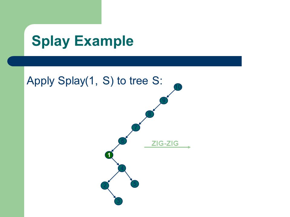
Splay Example Apply Splay(1, S) to tree S: ZIG-ZIG 10 9 8 7 6 5 4 3 2
 to tree S: ZIG-ZIG")
168
Splay Example Apply Splay(1, S) to tree S: ZIG-ZIG 10 9 8 7 6 5 4 1 2
3

169
Splay Example Apply Splay(1, S) to tree S: ZIG-ZIG 10 9 8 7 6 1 4 5 2
3 4 5
170
Splay Example Apply Splay(1, S) to tree S: ZIG-ZIG 10 9 8 1 6 4 7 2 5
3

171
Splay Example Apply Splay(1, S) to tree S: 10 1 8 9 6 7 2 3 4 5 ZIG
 to tree S: ZIG")
172
Splay Example Apply Splay(1, S) to tree S: 1 10 8 9 6 7 2 3 4 5
 to tree S:")
173
Apply Splay(2, S) to tree S:
1 2 10 1 8 8 4 10 6 9 3 6 9 Splay(2) 4 7 5 7 2 5 3
")
174
Splay Tree Analysis Definitions.
Let S(x) denote subtree of S rooted at x. |S| = number of nodes in tree S. (S) = rank = log |S| . (x) = (S(x)). 2 S(8) 1 8 |S| = 10 (2) = 3 (8) = 3 (4) = 2 (6) = 1 (5) = 0 4 10 3 6 9 5 7
 denote subtree of S rooted at x. |S| = number of nodes in tree S. (S) = rank = log |S| . (x) = (S(x)). 2. S(8) |S| = 10. (2) = 3. (8) = 3. (4) = 2. (6) = 1. (5) =")
175
Splay Tree Analysis Define the potential function

176
Splay Tree Analysis Define the potential function
Associate a positive weight to each node v: w(v)
")
177
Splay Tree Analysis Define the potential function
Associate a positive weight to each node v: w(v) W(v)= w(y), y belongs to a subtree rooted at v
 W(v)= w(y), y belongs to a subtree rooted at v.")
178
Splay Tree Analysis Define the potential function
Associate a positive weight to each node v: w(v) W(v)= w(y), y belongs to a subtree rooted at v Rank(v) = log W(v)
 W(v)= w(y), y belongs to a subtree rooted at v. Rank(v) = log W(v)")
179
Splay Tree Analysis Define the potential function
Associate a positive weight to each node v: w(v) W(v)= w(y), y belongs to a subtree rooted at v Rank(v) = log W(v) The tree potential is: rank(v) v
 W(v)= w(y), y belongs to a subtree rooted at v. Rank(v) = log W(v) The tree potential is: rank(v) v.")
180
Upper bound for the amortized time of a complete splay operation
To estimate the time of a splay operation we are going to use the number of rotations

181
Upper bound for the amortized time of a complete splay operation
To estimate the time of a splay operation we use the number of rotations Lemma: The amortized time for a complete splay operation of a node x in a tree of root r is, at most, 1 + 3[rank(r) – rank(x)]
 – rank(x)]")
182
Upper bound for the amortized time of a complete splay operation
Proof: The amortized cost a is given by a=t + after – before t : number of rotations executed in the splaying

183
Upper bound for the amortized time of a complete splay operation
Proof: The amortized cost a is given by a=t + after – before a = o1 + o2 + o ok oi : amortized cost of the i-th operation during the splay ( zig or zig-zig or zig-zag)
")
184
Upper bound for the amortized time of a complete splay operation
Proof: i : potential function after i-th operation ranki : rank after i-th operation oi = ti + i – i-1

185
Splay Tree Analysis Operations Case 1: zig( zag)
Case 2: zig-zig (zag-zag) Case 3: zig-zag (zag-zig)
 Case 3: zig-zag (zag-zig)")
186
Splay Tree Analysis Case 1: Only one rotation (zig) root r x
 root r x")
187
Splay Tree Analysis Case 1: Only one rotation (zig) w.l.o.g. root r x
ZIG(x) A B B C
 A. B. B. C.")
188
Splay Tree Analysis Case 1: Only one rotation (zig) w.l.o.g.
root r x w.l.o.g. x r r x A C ZIG(x) A B B C After the operation only rank(x) and rank(r) change
 A. B. B. C. After the operation only rank(x) and rank(r) change.")
189
Splay Tree Analysis Since potential is the sum of every rank:
i - i-1 = ranki(r) + ranki(x) – ranki-1(r) – ranki-1(x)
 + ranki(x) – ranki-1(r) – ranki-1(x)")
190
Splay Tree Analysis Since potential is the sum of every rank:
i - i-1 = ranki(r) + ranki(x) – ranki-1(r) – ranki-1(x) ti = 1 (time of one rotation)
 + ranki(x) – ranki-1(r) – ranki-1(x) ti = 1 (time of one rotation)")
191
Splay Tree Analysis Since potential is the sum of every rank:
i - i-1 = ranki(r) + ranki(q) – ranki-1(r) – ranki-1(q) ti = 1 (time of one rotation) Amort. Complexity: oi = 1 + ranki(r) + ranki(x) – ranki-1(r) – ranki-1(x)
 + ranki(q) – ranki-1(r) – ranki-1(q) ti = 1 (time of one rotation) Amort. Complexity: oi = 1 + ranki(r) + ranki(x) – ranki-1(r) – ranki-1(x)")
192
Splay Tree Analysis Amort. Complexity:
oi = 1 + ranki(r) + ranki(x) – ranki-1(r) – ranki-1(x) x r A r x C ZIG(x) A B B C
 + ranki(x) – ranki-1(r) – ranki-1(x) x. r. A. r. x. C. ZIG(x) A. B. B. C.")
193
Splay Tree Analysis Amort. Complexity:
oi = 1 + ranki(r) + ranki(x) – ranki-1(r) – ranki-1(x) ranki-1(r) ranki(r) x r A r x C ZIG(x) A B B C ranki(x) ranki-1(x)
 + ranki(x) – ranki-1(r) – ranki-1(x) ranki-1(r) ranki(r) x. r. A. r. x. C. ZIG(x) A. B. B. C. ranki(x) ranki-1(x)")
194
Splay Tree Analysis Amort. Complexity: oi = 1 + ranki(x) – ranki-1(x)
ranki-1(r) ranki(r) x r A r x C ZIG(x) A B B C ranki(x) ranki-1(x)
 ranki(r) x. r. A. r. x. C. ZIG(x) A. B. B. C. ranki(x) ranki-1(x)")
195
Splay Tree Analysis Amort. Complexity:
oi = [ ranki(x) – ranki-1(x) ] ranki-1(r) ranki(r) q r A r q C ZIG(x) A B B C ranki(q) ranki-1(q)
 – ranki-1(x) ] ranki-1(r) ranki(r) q. r. A. r. q. C. ZIG(x) A. B. B. C. ranki(q) ranki-1(q)")
196
Splay Tree Analysis Case 2: Zig-Zig D C B A D ZIG-ZIG C A B z z y x y

197
Splay Tree Analysis Case 2: Zig-Zig
oi = 2 + ranki(x) + ranki(y)+ranki(z) – ranki-1(x) – ranki-1(y) – ranki-1(z) z D C z B y A x y D ZIG-ZIG x C A B
 + ranki(y)+ranki(z) – ranki-1(x) – ranki-1(y) – ranki-1(z) z. D. C. z. B. y. A. x. y. D. ZIG-ZIG. x. C. A. B.")
198
Splay Tree Analysis Case 2: Zig-Zig ranki-1(z)= ranki(x)
oi = 2 + ranki(x) + ranki(y)+ranki(z) – ranki-1(x) – ranki-1(y) – ranki-1(z) z ranki-1(z)= ranki(x) D C z B y A x y D ZIG-ZIG x C A B
 + ranki(y)+ranki(z) – ranki-1(x) – ranki-1(y) – ranki-1(z) z. ranki-1(z)= ranki(x) D. C. z. B. y. A. x. y. D. ZIG-ZIG. x. C. A. B.")
199
Splay Tree Analysis Case 2: Zig-Zig oi = 2 + ranki(y)+ranki(z) – ranki-1(x) – ranki-1(y) z D C z B y A x y D ZIG-ZIG x C A B

200
Splay Tree Analysis Case 2: Zig-Zig oi = 2 + ranki(y)+ranki(z) – ranki-1(x) – ranki-1(y) ranki(x) ranki(y) ranki-1(y) ranki-1(x) z D C z B y A x y D ZIG-ZIG x C A B
 ranki-1(x) z. D. C. z. B. y. A. x. y. D. ZIG-ZIG. x. C. A. B.")
201
Splay Tree Analysis oi 2 + ranki(x)+ranki(z) – 2ranki-1(x)
Case 2: Zig-Zig oi 2 + ranki(x)+ranki(z) – 2ranki-1(x) Convexity of log z D C z B y A x y D ZIG-ZIG x C A B
+ranki(z) – 2ranki-1(x) Convexity of log. z. D. C. z. B. y. A. x. y. D. ZIG-ZIG. x. C. A. B.")
202
Splay Tree Analysis oi 3[ ranki(x) – ranki-1(x) ] Case 2: Zig-Zig D
B y A x y D ZIG-ZIG x C A B
![Splay Tree Analysis oi 3[ ranki(x) – ranki-1(x) ] Case 2: Zig-Zig D](http://slideplayer.com/slide/4064848/13/images/202/Splay+Tree+Analysis+oi+%EF%82%A3+3%5B+ranki%28x%29+%E2%80%93+ranki-1%28x%29+%5D+Case+2%3A+Zig-Zig+D.jpg "B. y. A. x. y. D. ZIG-ZIG. x. C. A. B.")
203
Splay Tree Analysis oi 3[ ranki(x) – ranki-1(x) ]
Case 3: Zig-Zag (same Analysis of case 2) oi 3[ ranki(x) – ranki-1(x) ]
![Splay Tree Analysis oi 3[ ranki(x) – ranki-1(x) ]](http://slideplayer.com/slide/4064848/13/images/203/Splay+Tree+Analysis+oi+%EF%82%A3+3%5B+ranki%28x%29+%E2%80%93+ranki-1%28x%29+%5D.jpg "Case 3: Zig-Zag (same Analysis of case 2) oi 3[ ranki(x) – ranki-1(x) ]")
204
Splay Tree Analysis a = o1 + o2 + ... + ok 3[rank(r)-rank(x)]+1
Putting the three cases together and telescoping a = o1 + o ok 3[rank(r)-rank(x)]+1
![Splay Tree Analysis a = o1 + o ok 3[rank(r)-rank(x)]+1](http://slideplayer.com/slide/4064848/13/images/204/Splay+Tree+Analysis+a+%3D+o1+%2B+o+ok+%EF%82%A3+3%5Brank%28r%29-rank%28x%29%5D%2B1.jpg "Putting the three cases together and telescoping. a = o1 + o ok 3[rank(r)-rank(x)]+1.")
205
Splay Tree Analysis For proving different types of results we must set the weights accordingly

206
Splay Tree Analysis Theorem. The cost of m accesses is O(m log n), where n is the number of items in the tree
, where n is the number of items in the tree.")
207
Splay Tree Analysis Theorem. The cost of m accesses is O(m log n), where n is the number of items in the tree Proof: Define every weight as 1/n. Then, the amortized cost is at most 3 log n + 1. | | is at most n log n Thus, by summing over all accesses we conclude that the cost is at most m log n + n log n

208
Static Optimality Theorem
Theorem: Let q(i) be the number of accesses to item i. If every item is accessed at least once, then total cost is at most
 be the number of accesses to item i. If every item is accessed at least once, then total cost is at most.")
209
Static Optimality Theorem
Proof. Assign a weight of q(i)/m to item i. Then, rank(r)=0 and rank(i) log(q(i)/m) Thus, 3[rank(r) – rank(i)] +1 3log(m/q(i)) + 1 In addition, || Thus,
/m to item i. Then, rank(r)=0 and rank(i) log(q(i)/m) Thus, 3[rank(r) – rank(i)] +1 3log(m/q(i)) + 1. In addition, || Thus,")
210
Static Optimality Theorem
Theorem: The cost of an optimal static binary search tree is

211
Static Finger Theorem Theorem: Let i,...,n be the items in the splay tree. Let the sequence of accesses be i1,...,im. If f is a fixed item, the total access time is

212
Static Finger Theorem || n log n
Proof. Assign a weight 1/(|i –f|+1)2 to item i. Then, rank(r)= O(1). rank(ij)=O( log( |ij – f +1|) Since the weight of every item is at least 1/n 2, then || n log n
2 to item i. Then, rank(r)= O(1). rank(ij)=O( log( |ij – f +1|) Since the weight of every item is at least 1/n 2, then. || n log n.")
213
Dynamic Optimality Conjecture
Conjecture Consider any sequence of successful accesses on an n-node search tree. Let A be any algorithm that carries out each access by traversing the path from the root to the node containing the accessed item, at a cost of one plus the depth of the node containing the item, and that between accesses performs an arbitrary number of rotations anywhere in the tree, at a cost of one per rotation. Then the total time to perform all the accesses by splaying is no more than O(n) plus a constant times the time required by the algorithm.
 plus a constant times the time required by the algorithm.")
214
Dynamic Optimality Conjecture
Dynamic optimality - almost. E. Demaine, D. Harmon, J. Iacono, and M. Patrascu. In Foundations of Computer Science (FOCS), 2004
,")
215
Insertion and Deletion
Most of the theorems hold !

216
Paris Kanellakis Theory and Practice Award Award 1999
Splay Tree Data Structure Daniel D.K. Sleator and Robert E. Tarjan Citation For their invention of the widely-used "Splay Tree" data structure.

Similar presentations
 AVL trees are balanced. An AVL Tree is a binary search tree such that.>")
 AVL trees are balanced. An AVL Tree is a binary search tree such that.>")


 COMP171. AVL Trees / Slide 2 * Data, a set of elements * Data structure, a structured set of elements, linear, tree, graph, … * Linear:>")


 running time on the find/insert/remove operations. Idea: keep the tree balanced.>")

 Lecture 17-18 COMP171 Fall 2006.>")
 Prof. Th. Ottmann.>")
