Download presentation
Presentation is loading. Please wait.

1
Single session analysis using FEAT
David Field Thanks to…. Tom Johnstone, Jason Gledhill, FMRIB The combined aim of today's lecture and practical session is for you to look at one of these images in FSL and understand what it means… FEAT stands for FMRI Expert Analysis Tool (not one of their better acronyms…but not as bad as FLOBS) A single session is one 4D functional time series acquired from one subject. If you have two subjects, or two sessions from a single session then this is “multi-session” FMRI – see next week. Note that it is still multi session if the same participants stayed in the scanner between sessions, i.e. you stopped the scanner and started it again. Single session analysis is also referred to as first level analysis, and multi-session analysis is also referred to as second level analysis or higher level analysis. (you can technically have 3rd and 4thlevel…)
 A single session is one 4D functional time series acquired from one subject. If you have two subjects, or two sessions from a single session then this is multi-session FMRI – see next week. Note that it is still multi session if the same participants stayed in the scanner between sessions, i.e. you stopped the scanner and started it again. Single session analysis is also referred to as first level analysis, and multi-session analysis is also referred to as second level analysis or higher level analysis. (you can technically have 3rd and 4thlevel…)")
2
Single “session” or “first level” FMRI analysis
In FMRI you begin with 1000’s of time courses, one for each voxel location Lots of “preprocessing” is applied to maximise the quality of the data Then, each voxel time course is modelled independently the model is a set of regressors (EV’s) that vary over time the same model is applied to every voxel time course if (part of) the model fits the voxel time course well the voxel is said to be “active” Define session here, and say that if the scanner is turned off and then started again for the same person you will need to do a second level analysis to combine the results of two first level analyses 241 256 250 234 242 260 254
 that vary over time. the same model is applied to every voxel time course. if (part of) the model fits the voxel time course well the voxel is said to be active Define session here, and say that if the scanner is turned off and then started again for the same person you will need to do a second level analysis to combine the results of two first level analyses")
3
Plan for today Detailed look at the process of modelling a single voxel time course The input is a voxel time course of image intensity values and the design matrix, which is made up of multiple EV’s The GLM is used to find the linear combination of EV’s that explains the most variance in the voxel time course The output is a PE for each EV in the design matrix Preprocessing of voxel time courses this topic probably only makes much sense if you understand 1) above, which is why I am breaking with tradition and covering this topic second rather than first Implementing a single session analysis in FSL using FEAT (workshop) Note: There is no formal meeting in week 3 of the course, but the room will be open for you to complete worksheets from today and last week at least one experienced FSL user will be here to help FEAT stands for FMRI Expert Analysis Tool (not one of their better acronyms…) Session means 1 run of the scanner. if you turn it off and then on again with the same subject you have two sessions, and the correct thing to do is to process them separately
 above, which is why I am breaking with tradition and covering this topic second rather than first. Implementing a single session analysis in FSL using FEAT (workshop) Note: There is no formal meeting in week 3 of the course, but the room will be open for you to complete worksheets from today and last week. at least one experienced FSL user will be here to help. FEAT stands for FMRI Expert Analysis Tool (not one of their better acronyms…) Session means 1 run of the scanner. if you turn it off and then on again with the same subject you have two sessions, and the correct thing to do is to process them separately.")
4
Preprocessing….

5
When you run the FEAT GUI you will see a window like this with a number of tabs running across the top. Today, as far as pre-stats is concerned we are NOT interested in BO Unwarping (this is an option you use if you have acquired a field map in the scanner. the field map is an image of the distortions in the magnetic field of the scanner that were caused by susceptibility artefacts etc at sinuses and ear canals. you can use it to unwarp EPI images so that their shape is more similar to the structural. it gets complex in practice) Intensity normalization is very out of fashion these days. It forces every FMRI volume to have the same mean intensity. Doh! What if one of them actually has higher mean intensity due to greater activation…this will always be turned off but grand mean scaling is still carried out so that you can compare subject 1 with subject 2 later. this is normalization across all volumes rather than between them, so relative differences in mean intensity between volumes are preserved Perfusion subtraction is used for ASL (arterial spin labelling) which require the acquisition of an entirely different kind of image from the scanner. MELODIC is a great way of finding all the sources of variation over time and space in your data using independent component analysis. it will find head motion artefacts just as readily as task related activation. You don’t supply any model, it just searches the data. But the output is hard to make use of… Motion correction was covered last week. The BET brain extraction option here is for the 4D functional series. You’d normally turn this on. Brain extraction for the structural image that will be used as the target for registration has to be performed by you, BEFORE you use FEAT to set up your processing pipeline. Today’s lecture will cover motion correction, slice timing correction, smoothing, and temporal filtering On the Misc tab you can find balloon help. If you want to know more about the options in the FEAT pipeline make sure this is turned on (make the small box yellow)
 Intensity normalization is very out of fashion these days. It forces every FMRI volume to have the same mean intensity. Doh! What if one of them actually has higher mean intensity due to greater activation…this will always be turned off but grand mean scaling is still carried out so that you can compare subject 1 with subject 2 later. this is normalization across all volumes rather than between them, so relative differences in mean intensity between volumes are preserved. Perfusion subtraction is used for ASL (arterial spin labelling) which require the acquisition of an entirely different kind of image from the scanner. MELODIC is a great way of finding all the sources of variation over time and space in your data using independent component analysis. it will find head motion artefacts just as readily as task related activation. You don’t supply any model, it just searches the data. But the output is hard to make use of… Motion correction was covered last week. The BET brain extraction option here is for the 4D functional series. You’d normally turn this on. Brain extraction for the structural image that will be used as the target for registration has to be performed by you, BEFORE you use FEAT to set up your processing pipeline. Today’s lecture will cover motion correction, slice timing correction, smoothing, and temporal filtering. On the Misc tab you can find balloon help. If you want to know more about the options in the FEAT pipeline make sure this is turned on (make the small box yellow)")
6
The BET brain extraction option refers to the 4D functional series
This will not run BET on the structural Normally turn this on Brain extraction for the structural image that will be used as the target for registration has to be performed by you, before you use FEAT to set up the processing pipeline

7
On the Misc tab you can toggle balloon help
Balloon help will tell you what most of the options mean if you hover the mouse over a button or tickbox But it gets annoying after a while If progress watcher is selected then FEAT opens a web browser that shows regular updates of the stage your analysis has reached

8
Motion Correction: MCFLIRT
Aims to make sure that there is a consistent mapping between voxel X,Y,Z position and actual anatomical locations Each image in the 4D series is registered using a 6 DOF rigid body spatial transform to the reference image (by default, the series mid point) This means every image apart from the reference image is moved slightly MCFLIRT plots the movements that were made as output Always remember that motion correction does not work perfectly, especially when motion is large. This is why I find it is really useful to keep scanning the same subjects repeatedly, rather than using fresh ones for every study. Experienced subjects become very comfortable in the scanner environment and learn to lie vey still. They also get better at paying attention to the task rather than the environment they are in. If I had to scan a population that was likely to move a lot I’d first use a biofeedbaack procedure in a mock scanner to “teach” them to lie still. If you are going to use PACE in the Reading scanner so that you remove motion as you go along by repositioning slices then you really should try to make sure you get the record of adjustments made out of SINGO, otherwise you will have no idea how much your participants actually moved. PACE will be more effective with short TR because the slice position adjustments are made more often.
 This means every image apart from the reference image is moved slightly. MCFLIRT plots the movements that were made as output. Always remember that motion correction does not work perfectly, especially when motion is large. This is why I find it is really useful to keep scanning the same subjects repeatedly, rather than using fresh ones for every study. Experienced subjects become very comfortable in the scanner environment and learn to lie vey still. They also get better at paying attention to the task rather than the environment they are in. If I had to scan a population that was likely to move a lot I’d first use a biofeedbaack procedure in a mock scanner to teach them to lie still. If you are going to use PACE in the Reading scanner so that you remove motion as you go along by repositioning slices then you really should try to make sure you get the record of adjustments made out of SINGO, otherwise you will have no idea how much your participants actually moved. PACE will be more effective with short TR because the slice position adjustments are made more often.")
9
MCFLIRT output Head rotation Head translation Total displacement
In most cases it is sufficient to look at the total displacement graph. You only need to look at the individual directions of translation and rotation if there is a problem in the total displacement plot. Points: The rotation and translation plots are absolute with respect to the reference image in the middle of the time course. That’s why you can see bigger differences from zero near the beginning and end of the plots. This participant had a lot of z motion (nodding of head producing z translation and rotation near start of scan) This contrasts with the total displacement plot, where you have both absolute and relative motion plots. The mean relative displacement is the net amount of motion between consecutive functional volumes. The relative plot is really important (next slide). When looking at the total displacement plot, the first thing you must do is look at the range of values on the y axis. FSL autoscales the y axis to fit the data, so a participant like the one depicted here who only moved a total of 0.5 mm or so in the whole session will look the same as one who moved 3 times as much. So, check the y axis first. If the scale on the y axis has a max of about a 1mm or less don’t worry about that participant. If it is 3mm you should worry. You have the option of entering the actual motion parameters to the GLM as regressors of no interest, but people disagree on whether this is worthwhile if you have also resampled the images to remove estimated motion. Adding motion parameters as regressors of no interest also uses up a lot of degrees of freedom in the data because you are adding 6 more regressors to the model. MELODIC ICA is also an interesting approach you could use if you needed to scan a population that was not good at keeping still. Total displacement
 This contrasts with the total displacement plot, where you have both absolute and relative motion plots. The mean relative displacement is the net amount of motion between consecutive functional volumes. The relative plot is really important (next slide). When looking at the total displacement plot, the first thing you must do is look at the range of values on the y axis. FSL autoscales the y axis to fit the data, so a participant like the one depicted here who only moved a total of 0.5 mm or so in the whole session will look the same as one who moved 3 times as much. So, check the y axis first. If the scale on the y axis has a max of about a 1mm or less don’t worry about that participant. If it is 3mm you should worry. You have the option of entering the actual motion parameters to the GLM as regressors of no interest, but people disagree on whether this is worthwhile if you have also resampled the images to remove estimated motion. Adding motion parameters as regressors of no interest also uses up a lot of degrees of freedom in the data because you are adding 6 more regressors to the model. MELODIC ICA is also an interesting approach you could use if you needed to scan a population that was not good at keeping still. Total displacement.")
10
The total displacement plot
displacement is calculated relative to the volume in the middle of the time series In this data set there were 120 volumes (TR), so the displacements are calculated relative to volume 60 in the series. Looking at the plot you can see that the absolute displacement tends to be greater at the start and end of the time series. This is simply because the middle point was arbitrarily chosen to be “zero”. This also explains why displacement is zero in the middle of the plot. Relative displacement is head position at each time point relative to the previous time point. Absolute displacement is relative to the reference image.
, so the displacements are calculated relative to volume 60 in the series. Looking at the plot you can see that the absolute displacement tends to be greater at the start and end of the time series. This is simply because the middle point was arbitrarily chosen to be zero . This also explains why displacement is zero in the middle of the plot. Relative displacement is head position at each time point relative to the previous time point. Absolute displacement is relative to the reference image.")
11
The total displacement plot
Why should you be particularly concerned about high values in the relative motion plot? Note that large jumps in the relative motion plot are a serious issue. This is because they are likely to be accompanied by distortions in the image that are not properly compensated for by motion correction procedures**. They will then add a big chunk to your error term in the GLM, or produce false activation. You can try modelling such “spikes” out of the data with a single regressor that has a value of 1 where there are spikes, or a 0 elsewhere. [Don’t convolve that regressor with an HRF]. Slow drifts in the absolute motion plot are less problematic because the motion correction algorithm can deal with them better. **Why is the image likely to be distorted around the point where there are spikes in the relative motion plot? Answer is because sudden head motion will have produced changes in the magnetic field and caused all sorts of small gradients as tissue type boundaries are moved through the magnetic field. These gradients in turn influence the t2 relaxation time and can do very odd things to the image. So that’s why sudden big motion causes more problems than just a spatial displacement of the image Something you should think about when comparing two groups (e.g. patients with normals) is do the two groups differ in how much they move, or the kind of motion they make in the scanner. If there were systematic differences in motion between the two groups it could conceivably produce false activation differences between them. The first thing to do is look at the range of values plotted on the y axis, because MCFLIRT auto-scales the y axis to the data range
 is do the two groups differ in how much they move, or the kind of motion they make in the scanner. If there were systematic differences in motion between the two groups it could conceivably produce false activation differences between them. The first thing to do is look at the range of values plotted on the y axis, because MCFLIRT auto-scales the y axis to the data range.")
12
Slice timing correction
Each slice in a functional image is acquired separately. Acquisition is normally interleaved, which prevents blending of signal from adjacent slices Assuming a TR of 3 seconds and, what is the time difference between the acquisition of adjacent slices? The answer is 1.5 sec, and this is independent of the number of slices. The blending of signal from adjacent slices that can occur with sequential top to bottom acquisition (or bottom to top) is caused by “spin history effects” A single functional brain area may span two or more slices
 is caused by spin history effects A single functional brain area may span two or more slices.")
13
Why are the different slice timings a problem?
The same temporal model (design matrix) is fitted to every voxel time course therefore, the model assumes that all the voxel values in a single functional volume were measured simultaneously Given that they are not measured simultaneously, what are the implications? Consider two voxels from adjacent slices both voxels are from the same functional brain area this time the TR is 1.5, but the slice order differed from the standard interleaved procedure, so there is a 1 sec time gap between acquisition of two voxels in the adjacent slices that cover the functional brain area
 is fitted to every voxel time course. therefore, the model assumes that all the voxel values in a single functional volume were measured simultaneously. Given that they are not measured simultaneously, what are the implications Consider two voxels from adjacent slices. both voxels are from the same functional brain area. this time the TR is 1.5, but the slice order differed from the standard interleaved procedure, so there is a 1 sec time gap between acquisition of two voxels in the adjacent slices that cover the functional brain area.")
14
Blue line = real HRF in response to a brief event at time 0
Blue squares: intensity values at a voxel first sampled at 0.5 sec, then every 1.5 sec thereafter (TR = 1.5) Red circles: intensity values at a voxel from an adjacent slice first sampled at 1.5 sec, then every 1.5 sec thereafter (TR = 1.5)
 Red circles: intensity values at a voxel from an adjacent slice first sampled at 1.5 sec, then every 1.5 sec thereafter (TR = 1.5)")
15
These are the two voxel time courses that are submitted to the model
Notice that one voxel time course has the peak activation at 6 sec after the stimulus, and the other one at 4.5 sec after the stimulus! This is quite a big gap, and the problem would be more severe if the TR was 2.5 or 3 sec. These are the two voxel time courses that are submitted to the model

16
These are the two voxel time courses that are submitted to the model
The model time course is yoked to the mid point of the volume acquisition (TR), so there will be a better fit for voxels in slices acquired at or near that time. Notice that one voxel time course has the peak activation at 6 sec after the stimulus, and the other one at 4.5 sec after the stimulus! This is quite a big gap, and the problem would be more severe if the TR was 2.5 or 3 sec. These are the two voxel time courses that are submitted to the model
, so there will be a better fit for voxels in slices acquired at or near that time. Notice that one voxel time course has the peak activation at 6 sec after the stimulus, and the other one at 4.5 sec after the stimulus! This is quite a big gap, and the problem would be more severe if the TR was 2.5 or 3 sec. These are the two voxel time courses that are submitted to the model.")
17
Slice timing solutions
Any ideas based on what was covered earlier? Including temporal derivatives of the main regressors in the model allows the model to be shifted in time to fit voxels in slices acquired far away from the mid point of the TR But, this makes it difficult to interpret the PE’s for the derivatives: do they represent slice timing, or do they represent variations in the underlying HRF? and, you end up having to use F contrasts instead of t contrasts (see later for why this is to be avoided if possible)
")
18
Slice timing solutions
Any ideas based on what was covered earlier? Use a block design with blocks long enough that the BOLD response is summated over a long time period But, Not all experimental stimuli / tasks can be presented in a block design So, another option is to shift the data from different slices in time by small amounts so that it is as if all slices were acquired at once this is what the preprocessing option in FEAT does

19
Shifting the data in time - caveats
But if the TR is 3 seconds, and you need to move the data for a given slice by, e.g., 1 sec, you don’t have a real data point to use get round this by interpolating the missing time points to allow whole voxel time courses to be shifted in time so effectively they were all sampled at once at the middle of the TR But… Interpolation works OK for short TR, but it does not work well for long TR (> 3 sec?) So this solution only works well when slice timing issues are relatively minor There is a debate about whether to do slice timing correction before or after motion correction FSL does motion correction first some people advise against any slice timing correction Generally, if you have an event related design then use it, but make sure you check carefully with the scanner technician what order your slices were acquired in! The following discussion is from Slice Timing FAQ Frequently Asked Questions - Slice Timing Correction SliceTimingPapers SliceTimingHowTos SliceTimingLinks 1. What is slice timing correction? What's the point? In multi-shot EPI (or spiral methods, which mimic them on this front), slices of your functional images are acquired throughout your TR. You therefore sample the BOLD signal at different layers of the brain at different time points. But you'd really like to have the signal for the whole brain from the same time point. If a given region that spans two slices, for example, all activates at once, you want to see what the signal looks like from the whole region at once; without correcting for slice timing, you might think the part of the region that was sampled later was more active than the part sampled earlier, when in fact you just sampled from the later one at a point closer to the peak of its HRF. What slice-timing correction does is, for each voxel, examine the timecourse and shift it by a small amount, interpolating between the points you ACTUALLY sampled to give you back the timecourse you WOULD have gotten had you sampled every voxel at exactly the same time. That way you can make the assumption, in your modeling, that every point in a given functional image is the actual signal from the same point in time. 2. How does it work? The standard algorithm for slice timing correction uses sinc interpolation between time points, which is accomplished by a Fourier transform of the signal at each voxel. The Fourier transform renders any signal as the sum of some collection of scaled and phase-shifted sine waves; once you have the signal in that form, you can simply shift all the sines on a given slice of the brain forward or backward by the appropriate amount to get the appropriate interpolation. There are a couple pitfalls to this technique, mainly around the beginning and end of your run, highlighted in Calhoun et. al below, but these have largely been accounted for in the currently available modules for slice timing correction in the major programs. 3. Are there different methods or alternatives and how well do they work? One alternative to doing slice-timing correction, detailed below in Henson et. al, is simply to model your data with an HRF that accounts for significant variability in when your HRFs onset - i.e., including regressors in your model that convolve your data with both a canonical HRF and with its first temporal derivative, which is accomplished with the 'hrf + temporal derivative' option in SPM. In terms of detecting sheer activation, this seems to be effective, despite the loss of some degrees of freedom in your model; however, your efficiency in estimating your HRF is very significantly reduced by this method, so if you're interested in early vs. late comparisons or timecourse data, this method isn't particularly useful. Another option might be to include slice-specific regressors in your model, but I don't know of any program that currently implements this option, or any papers than report on it... 4. When should you use it? Slice timing correction is primarily important in event-related experiments, and especially if you're interested in doing any kind of timecourse analysis, or any type of 'early-onset vs. late-onset' comparison. In event-related experiments, however, it's very important; Henson et. al show that aligning your model's timescale to the top or bottom slice can results in completely missing large clusters on the slice opposite to the reference slice without doing slice timing correction. This problem is magnified if you're doing interleaved EPI; any sequence that places adjacent slices at distant temporal points will be especially affected by this issue. Any event-related experiment should probably use it. 5. When is it a bad idea? It's never that bad an idea, but because the most your signal could be distorted is by one TR, this type of correction isn't as important in block designs. Blocks last for many TRs and figuring out what's happening at any given single TR is not generally a priority, and although the interpolation errors introduced by slice timing correction are generally small, if they're not needed, there's not necessarily a point to introducing them. But if you're interested in doing any sort of timecourse analysis (or if you're using interleaved EPI), it's probably worthwhile. 6. How do you know if it’s working? Henson et. al and both Van de Moortele papers below have images of slice-time-corrected vs. un-slice-time-corrected data, and they demonstrate signatures you might look for in your data. Main characteristics might be the absence of significant differences between adjacent slices. I hope to post some pictures here in the next couple weeks of the SPM sample data, analyzed with and without slice timing correction, to explore in a more obvious way. 7. At what point in the processing stream should you use it? This is the great open question about slice timing, and it's not super-answerable. Both SPM and AFNI recommend you do it before doing realignment/motion correction, but it's not entirely clear why. The issue is this: If you do slice timing correction before realignment, you might look down your non-realigned timecourse for a given voxel on the border of gray matter and CSF, say, and see one TR where the head moved and the voxel sampled from CSF instead of gray. This would results in an interpolation error for that voxel, as it would attempt to interpolate part of that big giant signal into the previous voxel. On the other hand, if you do realignment before slice timing correction, you might shift a voxel or a set of voxels onto a different slice, and then you'd apply the wrong amount of slice timing correction to them when you corrected - you'd be shifting the signal as if it had come from slice 20, say, when it actually came from slice 19, and shouldn't be shifted as much. There's no way to avoid all the error (short of doing a four-dimensional realignment process combining spatial and temporal correction - possibly coming soon), but I believe the current thinking is that doing slice timing first minimizes your possible error. The set of voxels subject to such an interpolation error is small, and the interpolation into another TR will also be small and will only affect a few TRs in the timecourse. By contrast, if one realigns first, many voxels in a slice could be affected at once, and their whole timecourses will be affected. I think that's why it makes sense to do slice timing first. That said, here's some articles from the SPM list that comment helpfully on this subject both ways, and there are even more if you do a search for "slice timing AND before" in the archives of the list. Thread from Rik Henson Argument from Geoff Aguirre Response to Aguirre from Ashburner 8. How should you choose your reference slice? You can choose to temporally align your slices to any slice you've taken, but keep in mind that the further away from the reference slice a given slice is, the more it's being interpolated. Any interpolation generates some small error, so the further away the slice, the more error there will be. For this reason, many people recommend using the middle slice of the brain as a reference, minimizing the possible distance away from the reference for any slice in the brain. If you have a structure you're interested in a priori, though - hippocampus, say - it may be wise to choose a slice close to that structure, to minimize what small interpolation errors may crop up. 9. Is there some systematic bias for slices far away from your reference slice, because they're always being sampled at a different point in their HRF than your reference slice is? That's basically the issue of interpolation error - the further away from your reference slice you are, the more error you're going to have in your interpolation - because your look at the "right" timepoint is a lot blurrier. If you never sample the slice at the top of the head at the peak of the HRF, the interpolation can't be perfect there if you're interpolating to a time when the HRF should be peaking - but hopefully you have enough information about your HRF in your experiment to get a good estimation from other voxels. It's another argument for choosing the middle slice in your image - you want to get as much brain as possible in an area of low interpolation error (close to the reference slice). 10. How can you be sure you're not introducing more noise with interpolation errors than you're taking out with the correction? Pretty good question. I don't know enough about signal processing and interpolation to say exactly how big the interpolation errors are, but the empirical studies below seem to show a significant benefit in detection by doing correction without adding much noise or many false positive voxels. Anyone have any other comments about this? CategoryFaq ‹ Segmentation Papers up Slice Timing HOWTO › Posted by admin on Wed, 04/30/ :06 Login to post comments Search Search this site: Navigation Recent posts User login Username: * Password: * Request new password C
 So this solution only works well when slice timing issues are relatively minor. There is a debate about whether to do slice timing correction before or after motion correction. FSL does motion correction first. some people advise against any slice timing correction. Generally, if you have an event related design then use it, but make sure you check carefully with the scanner technician what order your slices were acquired in! The following discussion is from Slice Timing FAQ. Frequently Asked Questions - Slice Timing Correction. SliceTimingPapers. SliceTimingHowTos. SliceTimingLinks. 1. What is slice timing correction What s the point In multi-shot EPI (or spiral methods, which mimic them on this front), slices of your functional images are acquired throughout your TR. You therefore sample the BOLD signal at different layers of the brain at different time points. But you d really like to have the signal for the whole brain from the same time point. If a given region that spans two slices, for example, all activates at once, you want to see what the signal looks like from the whole region at once; without correcting for slice timing, you might think the part of the region that was sampled later was more active than the part sampled earlier, when in fact you just sampled from the later one at a point closer to the peak of its HRF. What slice-timing correction does is, for each voxel, examine the timecourse and shift it by a small amount, interpolating between the points you ACTUALLY sampled to give you back the timecourse you WOULD have gotten had you sampled every voxel at exactly the same time. That way you can make the assumption, in your modeling, that every point in a given functional image is the actual signal from the same point in time. 2. How does it work The standard algorithm for slice timing correction uses sinc interpolation between time points, which is accomplished by a Fourier transform of the signal at each voxel. The Fourier transform renders any signal as the sum of some collection of scaled and phase-shifted sine waves; once you have the signal in that form, you can simply shift all the sines on a given slice of the brain forward or backward by the appropriate amount to get the appropriate interpolation. There are a couple pitfalls to this technique, mainly around the beginning and end of your run, highlighted in Calhoun et. al below, but these have largely been accounted for in the currently available modules for slice timing correction in the major programs. 3. Are there different methods or alternatives and how well do they work One alternative to doing slice-timing correction, detailed below in Henson et. al, is simply to model your data with an HRF that accounts for significant variability in when your HRFs onset - i.e., including regressors in your model that convolve your data with both a canonical HRF and with its first temporal derivative, which is accomplished with the hrf + temporal derivative option in SPM. In terms of detecting sheer activation, this seems to be effective, despite the loss of some degrees of freedom in your model; however, your efficiency in estimating your HRF is very significantly reduced by this method, so if you re interested in early vs. late comparisons or timecourse data, this method isn t particularly useful. Another option might be to include slice-specific regressors in your model, but I don t know of any program that currently implements this option, or any papers than report on it When should you use it Slice timing correction is primarily important in event-related experiments, and especially if you re interested in doing any kind of timecourse analysis, or any type of early-onset vs. late-onset comparison. In event-related experiments, however, it s very important; Henson et. al show that aligning your model s timescale to the top or bottom slice can results in completely missing large clusters on the slice opposite to the reference slice without doing slice timing correction. This problem is magnified if you re doing interleaved EPI; any sequence that places adjacent slices at distant temporal points will be especially affected by this issue. Any event-related experiment should probably use it. 5. When is it a bad idea It s never that bad an idea, but because the most your signal could be distorted is by one TR, this type of correction isn t as important in block designs. Blocks last for many TRs and figuring out what s happening at any given single TR is not generally a priority, and although the interpolation errors introduced by slice timing correction are generally small, if they re not needed, there s not necessarily a point to introducing them. But if you re interested in doing any sort of timecourse analysis (or if you re using interleaved EPI), it s probably worthwhile. 6. How do you know if it’s working Henson et. al and both Van de Moortele papers below have images of slice-time-corrected vs. un-slice-time-corrected data, and they demonstrate signatures you might look for in your data. Main characteristics might be the absence of significant differences between adjacent slices. I hope to post some pictures here in the next couple weeks of the SPM sample data, analyzed with and without slice timing correction, to explore in a more obvious way. 7. At what point in the processing stream should you use it This is the great open question about slice timing, and it s not super-answerable. Both SPM and AFNI recommend you do it before doing realignment/motion correction, but it s not entirely clear why. The issue is this: If you do slice timing correction before realignment, you might look down your non-realigned timecourse for a given voxel on the border of gray matter and CSF, say, and see one TR where the head moved and the voxel sampled from CSF instead of gray. This would results in an interpolation error for that voxel, as it would attempt to interpolate part of that big giant signal into the previous voxel. On the other hand, if you do realignment before slice timing correction, you might shift a voxel or a set of voxels onto a different slice, and then you d apply the wrong amount of slice timing correction to them when you corrected - you d be shifting the signal as if it had come from slice 20, say, when it actually came from slice 19, and shouldn t be shifted as much. There s no way to avoid all the error (short of doing a four-dimensional realignment process combining spatial and temporal correction - possibly coming soon), but I believe the current thinking is that doing slice timing first minimizes your possible error. The set of voxels subject to such an interpolation error is small, and the interpolation into another TR will also be small and will only affect a few TRs in the timecourse. By contrast, if one realigns first, many voxels in a slice could be affected at once, and their whole timecourses will be affected. I think that s why it makes sense to do slice timing first. That said, here s some articles from the SPM list that comment helpfully on this subject both ways, and there are even more if you do a search for slice timing AND before in the archives of the list. Thread from Rik Henson. Argument from Geoff Aguirre. Response to Aguirre from Ashburner. 8. How should you choose your reference slice You can choose to temporally align your slices to any slice you ve taken, but keep in mind that the further away from the reference slice a given slice is, the more it s being interpolated. Any interpolation generates some small error, so the further away the slice, the more error there will be. For this reason, many people recommend using the middle slice of the brain as a reference, minimizing the possible distance away from the reference for any slice in the brain. If you have a structure you re interested in a priori, though - hippocampus, say - it may be wise to choose a slice close to that structure, to minimize what small interpolation errors may crop up. 9. Is there some systematic bias for slices far away from your reference slice, because they re always being sampled at a different point in their HRF than your reference slice is That s basically the issue of interpolation error - the further away from your reference slice you are, the more error you re going to have in your interpolation - because your look at the right timepoint is a lot blurrier. If you never sample the slice at the top of the head at the peak of the HRF, the interpolation can t be perfect there if you re interpolating to a time when the HRF should be peaking - but hopefully you have enough information about your HRF in your experiment to get a good estimation from other voxels. It s another argument for choosing the middle slice in your image - you want to get as much brain as possible in an area of low interpolation error (close to the reference slice). 10. How can you be sure you re not introducing more noise with interpolation errors than you re taking out with the correction Pretty good question. I don t know enough about signal processing and interpolation to say exactly how big the interpolation errors are, but the empirical studies below seem to show a significant benefit in detection by doing correction without adding much noise or many false positive voxels. Anyone have any other comments about this CategoryFaq. ‹ Segmentation Papers up Slice Timing HOWTO › Posted by admin on Wed, 04/30/ :06. Login to post comments. Search. Search this site: Navigation. Recent posts. User login. Username: * Password: * Request new password. C.")
20
Temporal filtering Filtering in time and/or space is a long-established method in any signal detection process to help "clean up" your signal The idea is if your signal and noise are present at separable frequencies in the data, you can attenuate the noise frequencies and thus increase your signal to noise ratio 1. Why do filtering? What’s it buy you? Filtering in time and/or space is a long-established method in any signal detection process to help "clean up" your signal. The idea is if your signal and noise are present at separable frequencies in the data, you can attenuate the noise frequencies and thus increase your signal to noise ratio. One obvious way you might do this is by knocking out frequencies you know are too low to correspond to the signal you want - in other words, if you have an idea of how fast your signal might be oscillating, you can knock out noise that is oscillating much slower than that. In fMRI, noise like this can have a number of courses - slow "scanner drifts," where the mean of the data drifts up or down gradually over the course of the session, or physiological influences like changes in basal metabolism, or a number of other sources. This type of filtering is called "high-pass filtering," because we remove the very low frequencies and "pass through" the high frequencies. Doing this in the spatial domain would correspond to highlighting the edges of your image (preserving high-frequency information); in the temporal domain, it corresponds to "straightening out" any large bends or drifts in your timecourse. Removing linear drifts from a timecourse is the simplest possible high-pass filter. Another obvious way you might do this would be the opposite - knock out the frequencies you know are too high to correspond to your signal. This removes noise that is oscillating much faster than your signal from the data. This type of filtering is called "low-pass filtering," because we remove the very high frequencies and "pass through" the low frequencies. Doing this in the spatial domain is simply spatial smoothing (see SmoothingFaq); in the temporal domain, it corresponds to temporal smoothing. Low-pass filtering is much more controversial than high-pass filtering, a controversy explored by the papers in TemporalFilteringPapers. Finally, you could apply combinations of these filters to try and restrict the signal you detect to a specific band of frequencies, preserving only oscillations faster than a certain speed and slower than a certain speed. This is called "band-pass filtering," because we "pass through" a band of frequencies and filter everything else out, and is usually implemented in neuroimaging as simply doing both high-pass and low-pass filtering separately. In all of these cases, the goal of temporal filtering is the same: to apply our knowledge about what the BOLD signal "should" look like in the temporal domain in order to remove noise that is very unlikely to be part of the signal. This buys us better SNR, and a much better chance of detecting real activations and rejecting false ones. 2. What actually happens to my signal when I filter it? How about the design matrix? Filtering is a pretty standard mathematical operation, so all the major neuroimaging programs essentially do it the same way. We'll use high-pass as an example, as low-pass is no longer standard in most neuroimaging programs. At some point before model estimation, the program will ask the user to specify a cutoff parameter in Hz or seconds for the filter. If specified in seconds, this cutoff is taken to mean the period of interest of the experiment; frequencies that repeat over a timescale longer than the specified cutoff parameter are removed. Once the design matrix is constructed but before model estimation has begun, the program will filter each voxel's timecourse (the filter is generally based on some discrete cosine matrix) before submitting it to the model estimation - usually a very quick process. A graphical representation of the timecourse would show a "straightening out" of the signal timecourse - oftentime timecourses will have gradual linear drifts or quadratic drifts, or even higher frequency but still gradual bends, which are all flattened away after the filtering. Other, older methods for high-pass filtering simply included a set of increasing-frequency cosines in the design matrix (see Holmes et. al below), allowing them to "soak up" low-frequency variance, but this is generally not done explicitly any more. Low-pass filtering proceeds much the same way, but the design matrix is also usually filtered to smooth out any high frequencies present in it, as the signal to be detected will no longer have them. Low-pass filters are less likely to be specified merely with a lower-bound period-of-interest cutoff; oftentimes low-pass filters are constructed deliberately to have the same shape as a canonical HRF, to help highlight signal with that shape (as per the matched-filter theorem). 3. What’s good about high-pass filtering? Bad? High-pass filtering is relatively uncontroversial, and is generally accepted as a good idea for neuroimaging data. One big reason for this is that the noise in fMRI isn't white - it's disproportionately present in the low frequencies. There are several sources for this noise (see PhysiologyFaq and BasicStatisticalModelingFaq for discussions of some of them), and they're expressed in the timecourses sometimes as linear or higher-order drifts in the mean of the data, sometimes as slightly faster but still gradual oscillations (or both). What's good about high-pass filtering is that it's a straightforward operation that can attenuate that noise to a great degree. A number of the papers below study the efficacy of preprocessing steps, and generally it's found to significantly enhance one's ability to detect true activations. The one downside of high-pass filtering is that it can sometimes be tricky to select exactly what one's period of interest is. If you only have a single trial type with some inter-trial interval, then your period of interest of obvious - the time from one trial's beginning to the next - but what if you have three or four? Or more than that? Is it still the time from one trial to the next? Or the time from one trial to the next trial of that same type? Or what? Skudlarski et. al (TemporalFilteringPapers) point out that a badly chosen cutoff period can be significantly worse than the simplest possible temporal filtering, which would just be removing any linear drift from the data. If you try and detect an effect whose frequency is lower than your cutoff, the filter will probably knock it completely out, along with the noise. On the other hand, there's enough noise at low frequencies to almost guarantee that you wouldn't be able to detect most very slow anyways. Perfusion imaging does not suffer from this problem, one of its benefits - the noise spectrum for perfusion imaging appears to be quite flat. 4. What’s good about low-pass filtering? Bad? Low-pass filtering is much more controversial in MRI, and even in the face of mounting empirical evidence that it wasn't doing much good, the SPM group long offered some substantial and reasonable arguments in favor of it. The two big reasons offered in favor of low-pass filtering broke down as: The matched-filter theorem suggests filtering our timecourse with a filter shaped like an HRF should enhance signals of that shape relative to the noise, and We need to modify our general linear model to account for all the autocorrelation in fMRI noise; one way of doing that is by conditioning our data with a low-pass filter - essentially 'coloring' the noise spectrum, or introducing our own autocorrelations - and assuming that our introduced autocorrelation 'swamps' the existing autocorrelations, so that they can be ignored. (See BasicStatisticalModelingFaq for more on this.) This was a way of getting around early ignorance about the shape of the noise spectrum in fMRI and avoiding the computational burden of approximating the autocorrelation function for each model. Even as those burdens began to be overcome, Friston et. al (TemporalFilteringPapers) pointed out potential problems with pre-whitening the data as opposed to low-pass filtering, relating to potential biases of the analysis. However, the mounting evidence demonstrating the failure of low-pass filtering, as well as advances in computation speed enabling better ways of dealing with autocorrelation, seem to have won the day. In practice, low-pass filtering seems to have the effect of greatly reducing one's sensitivity to detecting true activations without significantly enhancing the ability to reject false ones (see Skudlarksi et. al, Della-Maggiore et. al on TemporalFilteringPapers). The problem with low-pass filtering seems to be that because noise is not independent from timepoint to timepoint in fMRI, 'smoothing' the timecourse doesn't suppress the noise but can, in fact, enhance it relative to the signal - it amplifies the worst of the noise and smooths the peaks of the signal out. Simulations with white noise show significant benefits from low-pass filtering, but with real, correlated fMRI noise, the filtering because counter-effective. Due to these results and a better sense now of how to correctly pre-whiten the timeseries noise, low-pass filtering is now no longer available in SPM2, nor is it allowed by standard methods in AFNI or BrainVoyager. 5. How do you set your cutoff parameter? Weeeeelll... this is one of those many messy little questions in fMRI that has been kind of arbitrarily hand-waved away, because there's not a good, simple answer for it. You'd to like to filter out as much noise as possible - particularly in the nasty part of the noise power spectrum where the noise power increases abruptly - without removing any important signal at all. But this can be a little trickier than it sounds. Roughly, a good rule of thumb might be to take the 'fundamental frequency' of your experiment - the time between one trial start and the next - and double or triple it, to make sure you don't filter out anything closer to your fundamental frequency. SPM99 (and earlier) had a formula built in that would try and calculate this number. But if you had a lot of trial types, and some types weren't repeated for very long periods of time, you'd often get filter sizes that were way too long (letting in too much noise). So in SPM2 they scrapped the formula and now issue a default filter size of 128 seconds for everybody, which isn't really any better of a solution. In general, default sizes of 100 or 128 seconds are pretty standard for most trial lengths (say, 8-45 seconds). If you have particularly short trials (less than 10 seconds) you could probably go shorter, maybe more like 60 or 48 seconds. But this is a pretty arbitrary part of the process. The upside is that it's hard to criticize an exact number that's in the right ballpark, so you probably won't get a paper rejected purely because your filter size was all wrong.
; in the temporal domain, it corresponds to straightening out any large bends or drifts in your timecourse. Removing linear drifts from a timecourse is the simplest possible high-pass filter. Another obvious way you might do this would be the opposite - knock out the frequencies you know are too high to correspond to your signal. This removes noise that is oscillating much faster than your signal from the data. This type of filtering is called low-pass filtering, because we remove the very high frequencies and pass through the low frequencies. Doing this in the spatial domain is simply spatial smoothing (see SmoothingFaq); in the temporal domain, it corresponds to temporal smoothing. Low-pass filtering is much more controversial than high-pass filtering, a controversy explored by the papers in TemporalFilteringPapers. Finally, you could apply combinations of these filters to try and restrict the signal you detect to a specific band of frequencies, preserving only oscillations faster than a certain speed and slower than a certain speed. This is called band-pass filtering, because we pass through a band of frequencies and filter everything else out, and is usually implemented in neuroimaging as simply doing both high-pass and low-pass filtering separately. In all of these cases, the goal of temporal filtering is the same: to apply our knowledge about what the BOLD signal should look like in the temporal domain in order to remove noise that is very unlikely to be part of the signal. This buys us better SNR, and a much better chance of detecting real activations and rejecting false ones. 2. What actually happens to my signal when I filter it How about the design matrix Filtering is a pretty standard mathematical operation, so all the major neuroimaging programs essentially do it the same way. We ll use high-pass as an example, as low-pass is no longer standard in most neuroimaging programs. At some point before model estimation, the program will ask the user to specify a cutoff parameter in Hz or seconds for the filter. If specified in seconds, this cutoff is taken to mean the period of interest of the experiment; frequencies that repeat over a timescale longer than the specified cutoff parameter are removed. Once the design matrix is constructed but before model estimation has begun, the program will filter each voxel s timecourse (the filter is generally based on some discrete cosine matrix) before submitting it to the model estimation - usually a very quick process. A graphical representation of the timecourse would show a straightening out of the signal timecourse - oftentime timecourses will have gradual linear drifts or quadratic drifts, or even higher frequency but still gradual bends, which are all flattened away after the filtering. Other, older methods for high-pass filtering simply included a set of increasing-frequency cosines in the design matrix (see Holmes et. al below), allowing them to soak up low-frequency variance, but this is generally not done explicitly any more. Low-pass filtering proceeds much the same way, but the design matrix is also usually filtered to smooth out any high frequencies present in it, as the signal to be detected will no longer have them. Low-pass filters are less likely to be specified merely with a lower-bound period-of-interest cutoff; oftentimes low-pass filters are constructed deliberately to have the same shape as a canonical HRF, to help highlight signal with that shape (as per the matched-filter theorem). 3. What’s good about high-pass filtering Bad High-pass filtering is relatively uncontroversial, and is generally accepted as a good idea for neuroimaging data. One big reason for this is that the noise in fMRI isn t white - it s disproportionately present in the low frequencies. There are several sources for this noise (see PhysiologyFaq and BasicStatisticalModelingFaq for discussions of some of them), and they re expressed in the timecourses sometimes as linear or higher-order drifts in the mean of the data, sometimes as slightly faster but still gradual oscillations (or both). What s good about high-pass filtering is that it s a straightforward operation that can attenuate that noise to a great degree. A number of the papers below study the efficacy of preprocessing steps, and generally it s found to significantly enhance one s ability to detect true activations. The one downside of high-pass filtering is that it can sometimes be tricky to select exactly what one s period of interest is. If you only have a single trial type with some inter-trial interval, then your period of interest of obvious - the time from one trial s beginning to the next - but what if you have three or four Or more than that Is it still the time from one trial to the next Or the time from one trial to the next trial of that same type Or what Skudlarski et. al (TemporalFilteringPapers) point out that a badly chosen cutoff period can be significantly worse than the simplest possible temporal filtering, which would just be removing any linear drift from the data. If you try and detect an effect whose frequency is lower than your cutoff, the filter will probably knock it completely out, along with the noise. On the other hand, there s enough noise at low frequencies to almost guarantee that you wouldn t be able to detect most very slow anyways. Perfusion imaging does not suffer from this problem, one of its benefits - the noise spectrum for perfusion imaging appears to be quite flat. 4. What’s good about low-pass filtering Bad Low-pass filtering is much more controversial in MRI, and even in the face of mounting empirical evidence that it wasn t doing much good, the SPM group long offered some substantial and reasonable arguments in favor of it. The two big reasons offered in favor of low-pass filtering broke down as: The matched-filter theorem suggests filtering our timecourse with a filter shaped like an HRF should enhance signals of that shape relative to the noise, and. We need to modify our general linear model to account for all the autocorrelation in fMRI noise; one way of doing that is by conditioning our data with a low-pass filter - essentially coloring the noise spectrum, or introducing our own autocorrelations - and assuming that our introduced autocorrelation swamps the existing autocorrelations, so that they can be ignored. (See BasicStatisticalModelingFaq for more on this.) This was a way of getting around early ignorance about the shape of the noise spectrum in fMRI and avoiding the computational burden of approximating the autocorrelation function for each model. Even as those burdens began to be overcome, Friston et. al (TemporalFilteringPapers) pointed out potential problems with pre-whitening the data as opposed to low-pass filtering, relating to potential biases of the analysis. However, the mounting evidence demonstrating the failure of low-pass filtering, as well as advances in computation speed enabling better ways of dealing with autocorrelation, seem to have won the day. In practice, low-pass filtering seems to have the effect of greatly reducing one s sensitivity to detecting true activations without significantly enhancing the ability to reject false ones (see Skudlarksi et. al, Della-Maggiore et. al on TemporalFilteringPapers). The problem with low-pass filtering seems to be that because noise is not independent from timepoint to timepoint in fMRI, smoothing the timecourse doesn t suppress the noise but can, in fact, enhance it relative to the signal - it amplifies the worst of the noise and smooths the peaks of the signal out. Simulations with white noise show significant benefits from low-pass filtering, but with real, correlated fMRI noise, the filtering because counter-effective. Due to these results and a better sense now of how to correctly pre-whiten the timeseries noise, low-pass filtering is now no longer available in SPM2, nor is it allowed by standard methods in AFNI or BrainVoyager. 5. How do you set your cutoff parameter Weeeeelll... this is one of those many messy little questions in fMRI that has been kind of arbitrarily hand-waved away, because there s not a good, simple answer for it. You d to like to filter out as much noise as possible - particularly in the nasty part of the noise power spectrum where the noise power increases abruptly - without removing any important signal at all. But this can be a little trickier than it sounds. Roughly, a good rule of thumb might be to take the fundamental frequency of your experiment - the time between one trial start and the next - and double or triple it, to make sure you don t filter out anything closer to your fundamental frequency. SPM99 (and earlier) had a formula built in that would try and calculate this number. But if you had a lot of trial types, and some types weren t repeated for very long periods of time, you d often get filter sizes that were way too long (letting in too much noise). So in SPM2 they scrapped the formula and now issue a default filter size of 128 seconds for everybody, which isn t really any better of a solution. In general, default sizes of 100 or 128 seconds are pretty standard for most trial lengths (say, 8-45 seconds). If you have particularly short trials (less than 10 seconds) you could probably go shorter, maybe more like 60 or 48 seconds. But this is a pretty arbitrary part of the process. The upside is that it s hard to criticize an exact number that s in the right ballpark, so you probably won t get a paper rejected purely because your filter size was all wrong.")
22
AAAAAAAVVVVVVVRRRRRRRAAAAAAAVVVVVVVRRRRRRR
For example, this real voxel time course has low frequency drift, high frequency noise, and maybe some signal at the period of the experimental design, but this is hidden by the sources of noise. In fMRI, the low frequency noise like can have a number of courses - slow "scanner drifts," where the mean of the data drifts up or down gradually over the course of the session, or physiological influences like changes in basal metabolism, or a number of other sources. We do not generally attempt to filter out the high frequency noise because this has nasty unintended consequences. See temporal autocorrelation later.

23
AAAAAAAVVVVVVVRRRRRRRAAAAAAAVVVVVVVRRRRRRR Time
A = auditory stimulation V = visual stimulation R = Rest block Block last about 16 seconds each. The experiment has a periodic (repetitive) structure in time. One cycle of the experiment is the first 3 blocks in this example. If a voxel had a time course that looked like the top image it would be oscillating at a period much higher than the experimental period. If a voxel had a time course that looked like the middle on it would be oscillating at a period much lower than the experimental period (assuming it eventually begins to rise again) If a voxel had a time course like the bottom one it would have a period very similar to the experimental time course, and its period would be peaking on the Visual block – looks like a visual cortex voxel! The problem is that the activation of a voxel often looks like the sum of these 3 lines!
 structure in time. One cycle of the experiment is the first 3 blocks in this example. If a voxel had a time course that looked like the top image it would be oscillating at a period much higher than the experimental period. If a voxel had a time course that looked like the middle on it would be oscillating at a period much lower than the experimental period (assuming it eventually begins to rise again) If a voxel had a time course like the bottom one it would have a period very similar to the experimental time course, and its period would be peaking on the Visual block – looks like a visual cortex voxel! The problem is that the activation of a voxel often looks like the sum of these 3 lines!")
24
Raw data Data from my replication and extension of Angelo Mosso (1870) “Using a lever to measure changes in cerebral blood volume related to mental activity”
 Using a lever to measure changes in cerebral blood volume related to mental activity")
25
After low pass filter Low pass filter was 6 second hanning window

26
Very low frequency component, suggests that high pass filter also needed
If you remove some low frequencies and some high frequencies to leave a range in the middle this is band-pass filtering. I knew that this slow drift could not be stimulus related because the stimulus was occurring every 25 sec, and this trend has a period of about 6 minutes!

27
Low and high frequencies removed
If you compare this plot with the raw data plot you can see intuitively that a lot of the noise is removed. By this I mean that the standard deviation across time is much reduced. In this data there was a stimulus presented once every 25 sec for 10 minutes. I removed frequencies that were higher and lower than these frequencies. removing high and low is called band pass filtering

28
Setting the high pass filter for FMRI
The rule recommended by FSL is that the lowest setting for the high pass filter should be equal to the duration of a single cycle of the design In an ABCABCABC block design, it will be equal to ABC If you set a shorter duration than this you will remove signal that is associated with the experiment If you set a higher duration than this then any unsystematic variation (noise) in the data with a periodic structure lower in frequency than the experimental cycle time will remain in voxel time courses In complicated event related designs lacking a strongly periodic structure there is a subjective element to the setting of the high pass filter The one downside of high-pass filtering is that it can sometimes be tricky to select exactly what one's period of interest is. If you only have a single trial type with some inter-trial interval, then your period of interest of obvious - the time from one trial's beginning to the next - but what if you have three or four? Or more than that? Is it still the time from one trial to the next? Or the time from one trial to the next trial of that same type? Or what? Skudlarski et. al (TemporalFilteringPapers) point out that a badly chosen cutoff period can be significantly worse than the simplest possible temporal filtering, which would just be removing any linear drift from the data. If you try and detect an effect whose frequency is lower than your cutoff, the filter will probably knock it completely out, along with the noise. On the other hand, there's enough noise at low frequencies to almost guarantee that you wouldn't be able to detect most very slow experimentally induced oscillations anyways. Perfusion imaging does not suffer from this problem, one of its benefits - the noise spectrum for perfusion imaging appears to be quite flat.
 in the data with a periodic structure lower in frequency than the experimental cycle time will remain in voxel time courses. In complicated event related designs lacking a strongly periodic structure there is a subjective element to the setting of the high pass filter. The one downside of high-pass filtering is that it can sometimes be tricky to select exactly what one s period of interest is. If you only have a single trial type with some inter-trial interval, then your period of interest of obvious - the time from one trial s beginning to the next - but what if you have three or four Or more than that Is it still the time from one trial to the next Or the time from one trial to the next trial of that same type Or what Skudlarski et. al (TemporalFilteringPapers) point out that a badly chosen cutoff period can be significantly worse than the simplest possible temporal filtering, which would just be removing any linear drift from the data. If you try and detect an effect whose frequency is lower than your cutoff, the filter will probably knock it completely out, along with the noise. On the other hand, there s enough noise at low frequencies to almost guarantee that you wouldn t be able to detect most very slow experimentally induced oscillations anyways. Perfusion imaging does not suffer from this problem, one of its benefits - the noise spectrum for perfusion imaging appears to be quite flat.")
29
Setting the high pass filter for FMRI
Do not use experimental designs with many conditions where the duration of a single experimental cycle is very long e.g. ABCDEABCDE, where ABCDE = 300 seconds setting the high pass to 300 sec will allow a lot of the low frequency FMRI noise to pass through to the modelling stage Furthermore, the noise can easily become correlated with the experimental time course because you are using an experimental time course that has a similar frequency to that of FMRI noise In any signal detection experiment, not just FMRI, you need to ensure that the signal of interest and noise are present at different temporal frequencies The one downside of high-pass filtering is that it can sometimes be tricky to select exactly what one's period of interest is. If you only have a single trial type with some inter-trial interval, then your period of interest of obvious - the time from one trial's beginning to the next - but what if you have three or four? Or more than that? Is it still the time from one trial to the next? Or the time from one trial to the next trial of that same type? Or what? Skudlarski et. al (TemporalFilteringPapers) point out that a badly chosen cutoff period can be significantly worse than the simplest possible temporal filtering, which would just be removing any linear drift from the data. If you try and detect an effect whose frequency is lower than your cutoff, the filter will probably knock it completely out, along with the noise. On the other hand, there's enough noise at low frequencies to almost guarantee that you wouldn't be able to detect most very slow experimentally induced oscillations anyways. Perfusion imaging does not suffer from this problem, one of its benefits - the noise spectrum for perfusion imaging appears to be quite flat.
 point out that a badly chosen cutoff period can be significantly worse than the simplest possible temporal filtering, which would just be removing any linear drift from the data. If you try and detect an effect whose frequency is lower than your cutoff, the filter will probably knock it completely out, along with the noise. On the other hand, there s enough noise at low frequencies to almost guarantee that you wouldn t be able to detect most very slow experimentally induced oscillations anyways. Perfusion imaging does not suffer from this problem, one of its benefits - the noise spectrum for perfusion imaging appears to be quite flat.")
30
Low pass filter? As well as removing oscillations with a longer cycle time than the experiment, you can also elect to remove oscillations with a higher cycle time than the experiment high frequency noise In theory this should enhance signal and reduce noise, and it was practiced in the early days of FMRI However, it has now been demonstrated that because FMRI noise has temporal structure (i.e. it is not white noise), the low pass filter can actually enhance noise relative to signal The temporal structure in the noise is called “temporal autocorrelation” and is dealt with in FSL using FILM prewhitening instead of low pass filtering in another break with the traditional structure of FMRI courses temporal autocorrelation and spatial smoothing will be covered after t and F contrasts However, the mounting evidence demonstrating the failure of low-pass filtering, as well as advances in computation speed enabling better ways of dealing with autocorrelation, seem to have won the day. In practice, low-pass filtering seems to have the effect of greatly reducing one's sensitivity to detecting true activations without significantly enhancing the ability to reject false ones (see Skudlarksi et. al, Della-Maggiore et. al on TemporalFilteringPapers). The problem with low-pass filtering seems to be that because noise is not independent from timepoint to timepoint in fMRI, 'smoothing' the timecourse doesn't suppress the noise but can, in fact, enhance it relative to the signal - it amplifies the worst of the noise and smooths the peaks of the signal out. Simulations with white noise show significant benefits from low-pass filtering, but with real, correlated fMRI noise, the filtering because counter-effective. Due to these results and a better sense now of how to correctly pre-whiten the timeseries noise, low-pass filtering is now no longer available in SPM2, nor is it allowed by standard methods in AFNI or BrainVoyager.
, the low pass filter can actually enhance noise relative to signal. The temporal structure in the noise is called temporal autocorrelation and is dealt with in FSL using FILM prewhitening instead of low pass filtering. in another break with the traditional structure of FMRI courses temporal autocorrelation and spatial smoothing will be covered after t and F contrasts. However, the mounting evidence demonstrating the failure of low-pass filtering, as well as advances in computation speed enabling better ways of dealing with autocorrelation, seem to have won the day. In practice, low-pass filtering seems to have the effect of greatly reducing one s sensitivity to detecting true activations without significantly enhancing the ability to reject false ones (see Skudlarksi et. al, Della-Maggiore et. al on TemporalFilteringPapers). The problem with low-pass filtering seems to be that because noise is not independent from timepoint to timepoint in fMRI, smoothing the timecourse doesn t suppress the noise but can, in fact, enhance it relative to the signal - it amplifies the worst of the noise and smooths the peaks of the signal out. Simulations with white noise show significant benefits from low-pass filtering, but with real, correlated fMRI noise, the filtering because counter-effective. Due to these results and a better sense now of how to correctly pre-whiten the timeseries noise, low-pass filtering is now no longer available in SPM2, nor is it allowed by standard methods in AFNI or BrainVoyager.")
31
After preprocessing and model fitting
You can now begin to answer the questions you set out to answer….

32
Which voxels “activated” in each experimental condition?
In the auditory / visual stimulus experiment, how do you decide if a voxel was more “activated” during the visual stimulus than the baseline? If the visual condition PE is > 0 then the voxel is active but > 0 has to take into account the noise in the data We need to be confident that if you repeated the experiment many times the PE would nearly always be > 0 How can you take the noise into account and quantify confidence that PE > 0? PE / residual variation in the voxel time course this is a t statistic, which can be converted to a p value by taking into account the degrees of freedom The p value is the probability of a PE as large or larger than the observed PE if the true value of the PE was 0 (null hypothesis) and the only variation present in the data was random variation FSL converts t statistics to z scores, simplifying interpretation because z can be converted to p without using deg of freedom Note that PE is also referred to as beta weight. The residual variation is represented by the standard error Dividing PE by residual variation is like dividing signal by noise, so you are basically expressing the variation in the time course you can account for in units of the variation of the time course that you cannot account for. As well as allowing conversion to a p value, this processing step also standardizes the different voxel time courses into units that are comparable across voxels. This is useful because some voxel time courses have a lot more variation in than others for reasons to do with the scanner, e.g. distance from the receiver coil – overall signal variation amplitude is larger nearer the receiver coil. Therefore bits of cortex nearer the middle of the brain, such as superior colliculus, have lower signal amplitude. Therefore standardisation across voxels is an important step. You would not be able to meaningfully compare the raw PE values for two voxels, but you can meaningfully compare the values of the two voxels if you first standardize into units of variability.
 and the only variation present in the data was random variation. FSL converts t statistics to z scores, simplifying interpretation because z can be converted to p without using deg of freedom. Note that PE is also referred to as beta weight. The residual variation is represented by the standard error. Dividing PE by residual variation is like dividing signal by noise, so you are basically expressing the variation in the time course you can account for in units of the variation of the time course that you cannot account for. As well as allowing conversion to a p value, this processing step also standardizes the different voxel time courses into units that are comparable across voxels. This is useful because some voxel time courses have a lot more variation in than others for reasons to do with the scanner, e.g. distance from the receiver coil – overall signal variation amplitude is larger nearer the receiver coil. Therefore bits of cortex nearer the middle of the brain, such as superior colliculus, have lower signal amplitude. Therefore standardisation across voxels is an important step. You would not be able to meaningfully compare the raw PE values for two voxels, but you can meaningfully compare the values of the two voxels if you first standardize into units of variability.")
33
Why include “effects of no interest” in the model?
Also called “nuisance regressors” Imagine an experiment about visual processing of faces versus other classes of object Why add EV’s to the design matrix based on the time course of: head motion parameters image intensity spikes physiological variables galvanic skin response, heart rate, pupil diameter Answer: to reduce the size of the residual error term t will be bigger when PE is bigger, but t will also be bigger when error is smaller You can model residual variation that is systematic in some way, but some of the residual variation is truly random in nature, e.g. thermal noise from the scanner, and cannot be modelled out galvanic skin response is an index of the intensity of emotional feeling, and has been used for lie detection. Pupil diameter is larger if you are paying more attention (assuming light levesl are equal in both conditions as pupil diameter mainly responds to light levels). Note that if you included a large number of regressors with periodic variation spanning a range of temporal frequencies you probably could model a lot of the random noise, but you’d burn up so may degrees of freedom that it would be self defeating. A model with excessive free (estimated) parameters is sometimes referred to as “over fitting”. Fourier basis set can end up like this if you are not careful.
. Note that if you included a large number of regressors with periodic variation spanning a range of temporal frequencies you probably could model a lot of the random noise, but you’d burn up so may degrees of freedom that it would be self defeating. A model with excessive free (estimated) parameters is sometimes referred to as over fitting . Fourier basis set can end up like this if you are not careful.")
34
t contrasts Contrast is short for Contrast of Parameter Estimates (COPE) it means a linear sum of PE’s. The simplest examples are implicit contrasts of individual PE’s with baseline. Using the example from the interactive spreadsheet visual PE * 1 + auditory PE * 0 visual PE * 0 + auditory PE * 1 To locate voxels where the visual PE is larger than the auditory PE visual PE * 1 + auditory PE * -1 To locate voxels where the auditory PE is larger than the visual PE visual PE * -1 + auditory PE * 1

35
t contrasts The value of the contrast in each voxel is divided by an estimate of the residual variation in the voxel time course (standard error) produces a t statistic of the contrast residual variation is based on the raw time course values minus the predicted values from the fitted model Activation maps (red and yellow blobs superimposed on anatomical images) are produced by mapping the t value at each voxel to a colour crudely, thresholding is just setting a value of t below which no colour is assigned. Note, the standard error is not the total variation divided by the number of TR (functional volumes). You divide by a somewhat smaller number. This is because the values of voxel intensity at each time point are not independent of the values at previous time points, so the effective number of observations is less. Unless you “prewhiten” the noise, in which case DOF are equal to N-1. See temporal autocorrelation.
 are produced by mapping the t value at each voxel to a colour. crudely, thresholding is just setting a value of t below which no colour is assigned. Note, the standard error is not the total variation divided by the number of TR (functional volumes). You divide by a somewhat smaller number. This is because the values of voxel intensity at each time point are not independent of the values at previous time points, so the effective number of observations is less. Unless you prewhiten the noise, in which case DOF are equal to N-1. See temporal autocorrelation.")
36
What will the [1 1] contrast give you?
Note that FSL converts all its t statistics to z statistics – standard normal distribution stuff, where 2 = 2 SD from mean is p = 0.05 This is how you will see t contrasts in FSL. The weightings are placed under the appropriate column of the design matrix. You need to get used to seeing the regressors in this vertical format instead of the horizontal format you used in the interactive spreadsheet. Time is now on the vertical axis rather than the horizontal axis. Something to be aware of is that FSL rescales all the regressors before showing them in the design matrix. So if you set up one regressor with a mean of zero and min / max of -2 and 2, and then another one with the same time course but min and max of -10 and 10, they will look identical in the design matrix, though they will end up with different PE’s if fitted. Ask Laura why this can be a problem…. What will the [1 1] contrast give you?
![What will the [1 1] contrast give you](http://slideplayer.com/slide/3992261/13/images/36/What+will+the+%5B1+1%5D+contrast+give+you.jpg "Note that FSL converts all its t statistics to z statistics – standard normal distribution stuff, where 2 = 2 SD from mean is p = This is how you will see t contrasts in FSL. The weightings are placed under the appropriate column of the design matrix. You need to get used to seeing the regressors in this vertical format instead of the horizontal format you used in the interactive spreadsheet. Time is now on the vertical axis rather than the horizontal axis. Something to be aware of is that FSL rescales all the regressors before showing them in the design matrix. So if you set up one regressor with a mean of zero and min / max of -2 and 2, and then another one with the same time course but min and max of -10 and 10, they will look identical in the design matrix, though they will end up with different PE’s if fitted. Ask Laura why this can be a problem…. What will the [1 1] contrast give you")
37
F contrasts These can be used to find voxels that are active in any one or more of a set of t contrasts Visual Auditory Tactile F contrasts are bidirectional (1 -1 also implies -1 1) rarely a good thing in practice….. If the response to an event was modelled with the standard HRF regressor plus time derivative then you can use an F contrast to view both components of model of the response to the event on a single activation map If you are relying on the time derivative to deal with slice timing correction then you are strongly advised to do this You can think of the F contrast as implementing a logical OR between the rows. The bidirectionality of F contrasts is a problem because most hypotheses are of the one tailed form “brain area X will have higher activation in experimental condition 1 than condition 2”, not “brain area X will either be more or less active in 1 than 2”. In practice you can use contrast masking, or looking at the time course of fitted model to figure out the direction of an effect. The reason you should be using an F contrast if you include time PE in a voxel is quite high for the time deriv, and only moderate for the normal regressor then you could miss activation if you just run a t contrast on the normal regressor. If you are only relying on the time derivatives to mop up a bit of noise in your data by taking account of slight differences in the HRF peak time between individuals and brain regions then you might be fine with t contrasts on the normal regressors only (Friston says it is Ok!). The lesson is probably to look at the results for the time derivatives if you included them in the model – too often they are ignored.
 rarely a good thing in practice….. If the response to an event was modelled with the standard HRF regressor plus time derivative then you can use an F contrast to view both components of model of the response to the event on a single activation map. If you are relying on the time derivative to deal with slice timing correction then you are strongly advised to do this. You can think of the F contrast as implementing a logical OR between the rows. The bidirectionality of F contrasts is a problem because most hypotheses are of the one tailed form brain area X will have higher activation in experimental condition 1 than condition 2 , not brain area X will either be more or less active in 1 than 2 . In practice you can use contrast masking, or looking at the time course of fitted model to figure out the direction of an effect. The reason you should be using an F contrast if you include time PE in a voxel is quite high for the time deriv, and only moderate for the normal regressor then you could miss activation if you just run a t contrast on the normal regressor. If you are only relying on the time derivatives to mop up a bit of noise in your data by taking account of slight differences in the HRF peak time between individuals and brain regions then you might be fine with t contrasts on the normal regressors only (Friston says it is Ok!). The lesson is probably to look at the results for the time derivatives if you included them in the model – too often they are ignored.")
38
Thresholding / multiple comparisons problem

39
Temporal autocorrelation
The image intensity value in a voxel at time X is partially predictable from the same voxel at times X-1, X-2, X-3 etc (even in baseline scans with no experiment) why is this a problem? it makes it hard to know the number of statistically independent observations in a voxel time course life would be simple if the number of observations was equal to the number of functional volumes temporal autocorrelation results in a true N is lower than this Why do we need to know the number of independent observations? because calculating a t statistic requires dividing by the standard error, and the standard error is SD / square root (N-1) Degrees of freedom are needed to convert t stats to p values If you use the number of time points in the voxel time course as N then p values will be too small (false positive) If we used number of volumes -1 for the DOF and standard error calculations, then we’d end up inflating our achieved statistical stignificance because the real number f independent observations in the time course is lower
 why is this a problem it makes it hard to know the number of statistically independent observations in a voxel time course. life would be simple if the number of observations was equal to the number of functional volumes. temporal autocorrelation results in a true N is lower than this. Why do we need to know the number of independent observations because calculating a t statistic requires dividing by the standard error, and the standard error is SD / square root (N-1) Degrees of freedom are needed to convert t stats to p values. If you use the number of time points in the voxel time course as N then p values will be too small (false positive) If we used number of volumes -1 for the DOF and standard error calculations, then we’d end up inflating our achieved statistical stignificance because the real number f independent observations in the time course is lower.")
40
Measuring autocorrelation

41
Measuring autocorrelation

42
Measuring autocorrelation

43
Measuring autocorrelation (SPSS style)
Note that in the correlation matrix you would make in SPSS from these numbers, you’d only be interested in looking at the correlations of the original time courses with the lagged time courses, not the correlations between different lags (so just one row of the matrix)
")
44
Plot the correlation against the degree of shift
Autocorrelation is seen most clearly in the residuals, once modelled sources of variation have been removed in the GLM stage. The correlation of the time course with the unshifted tme course (itself) is obviously going to be 1. If there was zero autocorrelation in the data you would see the gold line on the graph. In this case the temporal noise is white (equal power at every frequency) The red circle highlights the typical autocorrelation in FMRI data, which is strongest at lag 1, especially if you have a short TR. A long TR will avoid this problem to some extent. In this graph you can also see some negative autocorrelation at long lags (low temporal frequency). this suggests that no high pass filter was applied to this time course before the autocorrelation function was calculated. Or if it was filtered then the filter was not very efficient!
 is obviously going to be 1. If there was zero autocorrelation in the data you would see the gold line on the graph. In this case the temporal noise is white (equal power at every frequency) The red circle highlights the typical autocorrelation in FMRI data, which is strongest at lag 1, especially if you have a short TR. A long TR will avoid this problem to some extent. In this graph you can also see some negative autocorrelation at long lags (low temporal frequency). this suggests that no high pass filter was applied to this time course before the autocorrelation function was calculated. Or if it was filtered then the filter was not very efficient!")
45
Temporal autocorrelation
Generally, the value of a voxel at time t is partially predictable from nearby time points about 3-6 seconds in the past So, if you use a very long TR, e.g. 6, then you mostly avoid the problem as the original time points will have sufficient independence from each other Voxel values are also predictable from more distant time points due to low frequency noise with periodic structure but the high pass filter should deal with this problem FILM stands fro FMRIB’s improved linear modelling residuals = noise, hence the term prewhitening, because what you are doing is making the assumptions of the stats true by causing the residuals to have equal power at all temporal frequencies (in fourier terms) fMRI noise isn't white – and it's disproportionately present in the low frequencies. For this reason the high pass filter helps with the problem of autocorrelation that is present at low frequencies by removing some of the noise. But you still need to use FILM prewhitening. This is also a good reason to avoid fMRI experiments where the period of the experiment is very long (period = in an ABCABCABC design it is the time for ABC to occur, one cycle of the experiment) Posted by Tom Johnstone on July 09, 2002 at 11:54:48: In Reply to: temporal autocorrelation ? posted by Carl Senior on July 04, 2002 at 13:54:55: I'll have a crack at this, and allow Doug or others to correct any errors I make. Temporal autocorrelation refers to the correlation between time-shifted values of a voxel time series. It reflects the fact that the signal value at a given time point is not completely independent of its past signal values - indeed, there is a high dependence. The primary way in which this affects analysis is in the p-values quoted for individual subject analyses. These p-values are based in (large) part on the error degrees of freedom, which has to do with the number of *independent* observations that are used to calculate the statistic. The more independent obervations, the more powerful the statistical test, and the lower the p-value. The p-values reported in AFNI for single subject analyses assume that all time points are independent observations. But this is actually not the case, since their is temporal autocorrelation in the data. Thus the p-values reported will be too low, leading to the possibility of wrongly rejecting the null hypothesis. The solutions are varied. One solution is to use a much more conservative p-value as your criterion for rejecting the null hypothesis. This can be done either by rule of thumb, or, preferably, by using some sort of correction based on simulation using a null data set, or based on an estimate of the "effective" independent number of observations. Another option is to model the temporal autocorrelation explicitly (look up "linear mixed-models" on the web for more info on this). All of this becomes less relevant when pooling data across subjects for a group analysis, since then the error degrees of freedom in the statistical test is based upon the number of subjects, rather than the number of time points. . What is autocorrelation correction? Should I do it? The GLM approach suggested above and used for many types of experiments (not just neuroimaging) has a problem when applied to fMRI. It assumes that each observation is independent of the next, and any noise present at one timepoint is uncorrelated from the noise at the next timepoint. On that assumption, calculating the degrees of freedom in the data is easy - it's just the number of rows in the design matrix (number of TRs) minus the number of columns (number of effects), which makes calculating statistical significance for any beta value easy as well. The trouble with this assumption is that it's wrong for fMRI. The large bulk of the noise present in the fMRI signal is low-frequency noise, which is highly correlated from one timepoint to the next. From a spectral analysis point of view, the power spectrum of the noise isn't flat by a long shot - it's highly skewed to the low frequency. In other words, there is a high degree of autocorrelation in fMRI data - the value at each time point is significantly explained by the value at the timepoints before or after. This is a problem for estimating statistical significance, because it means that our naive calculation of degrees of freedom is wrong - there are fewer degrees of freedom in real life than if every timepoint were independent, because of the high level of correlation between time points. Timepoints don't vary completely freely - they are explained by the previous timepoints. So our effective degrees of freedom is smaller than our earlier guess - but in order to calculate how significant any beta value is, we need to know how much smaller. How can we do that? Friston and Worsley made an early attempt at this in the papers below. They argued that one way to account for the unknown autocorrelation was to essentially wash it out by applying their own, known, autocorrelation - temporally smoothing (or low-pass filtering) the data. The papers below extend the GLM framework to incorporate a known autocorrelation function and correctly calculate effective degrees of freedom for temporally smoothed data. This approach is sometimes called "coloring" the data - since uncorrelated noise is called "white" noise, this smoothing essentially "colors" the noise by rendering it less white. The idea is that after coloring, you know what color you've imposed, and so you can figure out exactly how to account for the color. SPM99 (and earlier) offer two forms of accounting for the autocorrelation - low-pass filtering and autocorrelation estimation (AR(1) model). The autocorrelation estimation corresponds more with pre-whitening (see below), although it's implemented badly in SPM99 and probably shouldn't be used. In practice, however, low-pass filtering seems to be a failure. Tests of real data have repeatedly shown that temporal smoothing of the data seems to hurt analysis sensitivity more than it helps, and harm false-positive rates more than it helps. The bias in fMRI noise is simply so significant that it can't be swamped without accounting for it. In real life, the proper theoretical approach seems to be pre-whitening, and low-pass filtering has been removed from SPM2 and continues to not be available in other major packages. (See TemporalFilteringFaq for more info.) 4. What is pre-whitening? How does it help? The other approach to dealing with autocorrelation in the fMRI noise power spectrum (see above), instead of 'coloring' the noise, is to 'whiten' it. If the GLM assumes white noise, the argument runs, let's make the noise we really have into white noise. This is generally how correlated noise is dealt with in the GLM literature, and it can be shown whitening the noise gives the most unbiased parameter estimates possible. The way to do this is simply by running a regreession on your data to find the extent of the autocorrelation. If you can figure out how much each timepoint's value is biased by the one before it, you can remove the effect of that previous timepoint, and that way only leave the 'white' part of the noise. In theory, this can be very tricky, because one doesn't actually know how many previous timepoints are influencing the current timepoint's value. Essentially, one is trying to model the noise, without having precise estimates of where the noise is coming from. In practice, however, enough work has been done on figuring out the sources of fMRI noise to have a fairly good model of what it looks like, and an AR(1) + w model, where each noise timepoint is some white noise plus a scaling of the noise timepoint before it, seems to be a good fit (it's also described as a 1/f model). This pre-whitening is available in SPM2 and BrainVoyager natively and can be applied to AFNI (I think). This procedure essentially estimates the level of autocorrelation (or 'color') in the noise, and removes it from the timeseries ('whitening' the noise).
 fMRI noise isn t white – and it s disproportionately present in the low frequencies. For this reason the high pass filter helps with the problem of autocorrelation that is present at low frequencies by removing some of the noise. But you still need to use FILM prewhitening. This is also a good reason to avoid fMRI experiments where the period of the experiment is very long (period = in an ABCABCABC design it is the time for ABC to occur, one cycle of the experiment) Posted by Tom Johnstone on July 09, 2002 at 11:54:48: In Reply to: temporal autocorrelation posted by Carl Senior on July 04, 2002 at 13:54:55: I ll have a crack at this, and allow Doug or others to correct any errors I make. Temporal autocorrelation refers to the correlation between time-shifted values of a voxel time series. It reflects the fact that the signal value at a given time point is not completely independent of its past signal values - indeed, there is a high dependence. The primary way in which this affects analysis is in the p-values quoted for individual subject analyses. These p-values are based in (large) part on the error degrees of freedom, which has to do with the number of *independent* observations that are used to calculate the statistic. The more independent obervations, the more powerful the statistical test, and the lower the p-value. The p-values reported in AFNI for single subject analyses assume that all time points are independent observations. But this is actually not the case, since their is temporal autocorrelation in the data. Thus the p-values reported will be too low, leading to the possibility of wrongly rejecting the null hypothesis. The solutions are varied. One solution is to use a much more conservative p-value as your criterion for rejecting the null hypothesis. This can be done either by rule of thumb, or, preferably, by using some sort of correction based on simulation using a null data set, or based on an estimate of the effective independent number of observations. Another option is to model the temporal autocorrelation explicitly (look up linear mixed-models on the web for more info on this). All of this becomes less relevant when pooling data across subjects for a group analysis, since then the error degrees of freedom in the statistical test is based upon the number of subjects, rather than the number of time points. . What is autocorrelation correction Should I do it The GLM approach suggested above and used for many types of experiments (not just neuroimaging) has a problem when applied to fMRI. It assumes that each observation is independent of the next, and any noise present at one timepoint is uncorrelated from the noise at the next timepoint. On that assumption, calculating the degrees of freedom in the data is easy - it s just the number of rows in the design matrix (number of TRs) minus the number of columns (number of effects), which makes calculating statistical significance for any beta value easy as well. The trouble with this assumption is that it s wrong for fMRI. The large bulk of the noise present in the fMRI signal is low-frequency noise, which is highly correlated from one timepoint to the next. From a spectral analysis point of view, the power spectrum of the noise isn t flat by a long shot - it s highly skewed to the low frequency. In other words, there is a high degree of autocorrelation in fMRI data - the value at each time point is significantly explained by the value at the timepoints before or after. This is a problem for estimating statistical significance, because it means that our naive calculation of degrees of freedom is wrong - there are fewer degrees of freedom in real life than if every timepoint were independent, because of the high level of correlation between time points. Timepoints don t vary completely freely - they are explained by the previous timepoints. So our effective degrees of freedom is smaller than our earlier guess - but in order to calculate how significant any beta value is, we need to know how much smaller. How can we do that Friston and Worsley made an early attempt at this in the papers below. They argued that one way to account for the unknown autocorrelation was to essentially wash it out by applying their own, known, autocorrelation - temporally smoothing (or low-pass filtering) the data. The papers below extend the GLM framework to incorporate a known autocorrelation function and correctly calculate effective degrees of freedom for temporally smoothed data. This approach is sometimes called coloring the data - since uncorrelated noise is called white noise, this smoothing essentially colors the noise by rendering it less white. The idea is that after coloring, you know what color you ve imposed, and so you can figure out exactly how to account for the color. SPM99 (and earlier) offer two forms of accounting for the autocorrelation - low-pass filtering and autocorrelation estimation (AR(1) model). The autocorrelation estimation corresponds more with pre-whitening (see below), although it s implemented badly in SPM99 and probably shouldn t be used. In practice, however, low-pass filtering seems to be a failure. Tests of real data have repeatedly shown that temporal smoothing of the data seems to hurt analysis sensitivity more than it helps, and harm false-positive rates more than it helps. The bias in fMRI noise is simply so significant that it can t be swamped without accounting for it. In real life, the proper theoretical approach seems to be pre-whitening, and low-pass filtering has been removed from SPM2 and continues to not be available in other major packages. (See TemporalFilteringFaq for more info.) 4. What is pre-whitening How does it help The other approach to dealing with autocorrelation in the fMRI noise power spectrum (see above), instead of coloring the noise, is to whiten it. If the GLM assumes white noise, the argument runs, let s make the noise we really have into white noise. This is generally how correlated noise is dealt with in the GLM literature, and it can be shown whitening the noise gives the most unbiased parameter estimates possible. The way to do this is simply by running a regreession on your data to find the extent of the autocorrelation. If you can figure out how much each timepoint s value is biased by the one before it, you can remove the effect of that previous timepoint, and that way only leave the white part of the noise. In theory, this can be very tricky, because one doesn t actually know how many previous timepoints are influencing the current timepoint s value. Essentially, one is trying to model the noise, without having precise estimates of where the noise is coming from. In practice, however, enough work has been done on figuring out the sources of fMRI noise to have a fairly good model of what it looks like, and an AR(1) + w model, where each noise timepoint is some white noise plus a scaling of the noise timepoint before it, seems to be a good fit (it s also described as a 1/f model). This pre-whitening is available in SPM2 and BrainVoyager natively and can be applied to AFNI (I think). This procedure essentially estimates the level of autocorrelation (or color ) in the noise, and removes it from the timeseries ( whitening the noise).")
46
Autocorrelation: FILM prewhitening
First, fit the model (regressors of interest and no interest) to the voxel time course using the GLM (ignoring the autocorrelation for the moment) Estimate the temporal autocorrelation structure in the residuals note: if model is good residuals = noise? The estimated structure can be inverted and used as a temporal filter to undo the autocorrelation structure in the original data the time points are now independent and so N = the number of time points (volumes) the filter is also applied to the design matrix Refit the GLM Run t and F tests with valid standard error and degrees of freedom Prewhitening is selected on the stats tab in FEAT it is computationally intensive, but with a modern PC it is manageable and there are almost no circumstances where you would turn this option off
 to the voxel time course using the GLM. (ignoring the autocorrelation for the moment) Estimate the temporal autocorrelation structure in the residuals. note: if model is good residuals = noise The estimated structure can be inverted and used as a temporal filter to undo the autocorrelation structure in the original data. the time points are now independent and so N = the number of time points (volumes) the filter is also applied to the design matrix. Refit the GLM. Run t and F tests with valid standard error and degrees of freedom. Prewhitening is selected on the stats tab in FEAT. it is computationally intensive, but with a modern PC it is manageable and there are almost no circumstances where you would turn this option off.")
47
Spatial smoothing FMRI noise varies across space as well as time
smoothing is a way of reducing spatial noise and thereby increasing the ratio of signal to noise (SNR) in the data Unlike FMRI temporal noise, FMRI spatial noise is more like white noise, making it easier to deal with it is essentially random, essentially independent from voxel to voxel, and has as mean of about zero therefore if you average image intensity across several voxels, noise tends to average towards zero, whereas signal that is common to the voxels you are averaging across will remain unchanged, dramatically improving the signal to noise ratio (SNR) A secondary benefit of smoothing is to reduce anatomical variation between participants that remains after registration to the template image this is because smoothing blurs the images that most of the spatial noise is (mostly) Gaussian - it's essentially random, essentially independent from voxel to voxel, and roughly centered around zero. If that's true, then if we average our intensity across several voxels, our noise will tend to average to zero, whereas our signal (which is some non-zero number) will tend to average to something non-zero, and presto! We've decreased our noise while not decreasing our signal, and our SNR is better. 1. What is smoothing? "Smoothing" is generally used to describe spatial smoothing in neuroimaging, and that's a nice euphamism for "blurring." Spatial smoothing consists of applying a small blurring kernel across your image, to average part of the intensities from neighboring voxels together. The effect is to blur the image somewhat and make it smoother - softening the hard edges, lowering the overall spatial frequency, and hopefully improving your signal-to-noise ratio. 2. What's the point of smoothing? Improving your signal to noise ratio. That's it, in a nutshell. This happens on a couple of levels, both the single-subject and the group. At the single-subject level: fMRI data has a lot of noise in it, but studies have shown that most of the spatial noise is (mostly) Gaussian - it's essentially random, essentially independent from voxel to voxel, and roughly centered around zero. If that's true, then if we average our intensity across several voxels, our noise will tend to average to zero, whereas our signal (which is some non-zero number) will tend to average to something non-zero, and presto! We've decreased our noise while not decreasing our signal, and our SNR is better. (Desmond & Glover (DesignPapers) demonstrate this effect with real data.) Matthew Brett has a nice discussion and several illustrations of this on the Cambridge Imagers page: At the group level: Anatomy is highly variable between individuals, and so is exact functional placement within that anatomy. Even with normalized data, there'll be some good chunk of variability between subjects as to where a given functional cluster might be. Smoothing will blur those clusters and thus maximize the overlap between subjects for a given cluster, which increases our odds of detecting that functional cluster at the group level and increasing our sensitivity. Finally, a slight technical note for SPM: Gaussian field theory, by which SPM does p-corrections, is based on how smooth your data is - the more spatial correlation in the data, the better your corrected p-values will look, because there's fewer degree of freedom in the data. So in SPM, smoothing will give you a direct bump in p-values - but this is not a "real" increase in sensitivity as such. FSL also uses gaussian field theory for voxelwise correction of multiple comparisons. 3. When should you smooth? When should you not? Smoothing is a good idea if: You're not particularly concerned with voxel-by-voxel resolution. You're not particularly concerned with finding small (less than a handful of voxels) clusters. You want (or need) to improve your signal-to-noise ratio. You're averaging results over a group, in a brain region where functional anatomy and organization isn't precisely known. You're using SPM, and you want to use p-values corrected with Gaussian field theory (as opposed to FDR). Smoothing'd not a good idea if: You need voxel-by-voxel resolution. You believe your activations of interest will only be a few voxels large. You're confident your task will generate large amounts of signal relative to noise. You're working primarily with single-subject results. You're mainly interested in getting region-of-interest data from very specific structures that you've drawn with high resolution on single subjects. 4. At what point in your analysis stream should you smooth? The first point at which it's obvious to smooth is as the last spatial preprocessing step for your raw images; smoothing before then will only reduce the accuracy of the earlier preprocessing (normalization, realignment, etc.) - those programs that need smooth images do their own smoothing in memory as part of the calculation, and don't save the smoothed versions. One could also avoid smoothing the raw images entirely and instead smooth the beta and/or contrast images. In terms of efficiency, there's not much difference - smoothing even hundreds of raw images is a very fast process. So the question is one of performance - which is better for your sensitivity? Skudlarski et. al (SmoothingPapers) evaluated this for single-subject data and found almost no difference between the two methods. They did find that multifiltering (see below) had greater benefits when the smoothing was done on the raw images as opposed to the statistical maps. Certainly if you want to use p-values corrected with Gaussian field theory (a la SPM), you need to smooth before estimating your results. It's a bit of a toss-up, though... 5. How do you determine the size of your kernel? Based on your resolution? Or structure size? A little of both, it seems. The matched filter theorem, from the signal processing field, tells us that if we're trying to recover a signal (like an activation) in noisy data (like fMRI), we can best do it by smoothing our data with a kernel that's about the same size as our activation. Trouble is, though, most of us don't know how big our activations are going to be before we run our experiment. Even if you have a particular structure of interest (say, the hippocampus), you may not get activation over the whole region - only a part. Given that ambiguity, Skudlarski et. al introduce a method called multifiltering, in which you calculate results once from smoothed images, and then a second set of results from unsmoothed images. Finally, you average together the beta/con images from both sets of results to create a final set of results. The idea is that the smoothed set of results preferentially highlight larger activations, while the unsmoothed set of results preserve small activations, and the final set has some of the advantages of both. Their evaluations showed multifiltering didn't detect larger activations (clusters with radii of 3-4 voxels or greater) as well as purely smoothed results (as you might predict) but that over several cluster sizes, multifiltering outperformed traditional smoothing techniques. Its use in your experiment depends on how important you consider detecting activations of small size (less than 3-voxel radius, or about). Overall, Skudlarski et. al found that over several cluster sizes, a kernel size of 1-2 voxels (3-6 mm, in their case) was most sensitive in general. A good rule of thumb is to avoid using a kernel that's significantly larger than any structure you have a particular a priori interest in, and carefully consider what your particular comfort level is with smaller activations. A 2-voxel-radius cluster is around 30 voxels and change (and multifiltering would be more sensitive to that size); a 3-voxel-radius cluster is 110 voxels or so (if I'm doing my math right). 6mm is a good place to start. If you're particularly interested in smaller activations, 2-4mm might be better. If you know you won't care about small activations and really will only look at large clusters, 8-10mm is a good range. 6. Should you use a different kernel for different parts of the brain? It's an interesting question. Hopfinger et. al find that a 6mm kernel works best for the data they examine in the cortex, but a larger kernel (10mm) works best in subcortical regions. This might be counterintuitive, considering the subcortical structures they examine are small in general than large cortical activations - but they unfortunately don't include information about the size of their activation clusters, so the results are difficult to interpret. You might think a smaller kernel in subcortical regions would be better, due to the smaller size of the structures. Trouble is, figuring out exactly which parts of the brain to use a different size of kernel on presupposes a lot of information - about activation size, about shape of HRF in one region vs. another - that pretty much doesn't exist for most experimental set-ups or subjects. I would tend to suggest that varying the size of the kernel for different regions is probably more trouble than it's worth at this point, but that may change as more studies come out about HRFs in different regions and individualized effects of smoothing. See Kiebel and Friston (SmoothingPapers), though, for some advanced work on changing the shape of the kernel in different regions... 7. What does it actually do to your activation data? About what you'd expect - preferentially brings out larger activations. Check out White et. al (SmoothingPapers) for some detailed illustrations. We hope to have some empirical results and maybe some pictures up here in the next few weeks... 8. What does it do to ROI data? Great question, and not one I've got a good answer for at the moment. One big part of the answer will depend on the ratio of your smoothing kernel size to your ROI size. Presumably, assuming your kernel size is smaller than your ROI, it may help improve SNR in your ROI, but if the kernel and ROI are similar sizes, smoothing may also blur the signal such that your structure contains less activation. With any luck, we can do a little empirical testing on this questions and have some results up here in the future...
 in the data. Unlike FMRI temporal noise, FMRI spatial noise is more like white noise, making it easier to deal with. it is essentially random, essentially independent from voxel to voxel, and has as mean of about zero. therefore if you average image intensity across several voxels, noise tends to average towards zero, whereas signal that is common to the voxels you are averaging across will remain unchanged, dramatically improving the signal to noise ratio (SNR) A secondary benefit of smoothing is to reduce anatomical variation between participants that remains after registration to the template image. this is because smoothing blurs the images. that most of the spatial noise is (mostly) Gaussian - it s essentially random, essentially independent from voxel to voxel, and roughly centered around zero. If that s true, then if we average our intensity across several voxels, our noise will tend to average to zero, whereas our signal (which is some non-zero number) will tend to average to something non-zero, and presto! We ve decreased our noise while not decreasing our signal, and our SNR is better. 1. What is smoothing Smoothing is generally used to describe spatial smoothing in neuroimaging, and that s a nice euphamism for blurring. Spatial smoothing consists of applying a small blurring kernel across your image, to average part of the intensities from neighboring voxels together. The effect is to blur the image somewhat and make it smoother - softening the hard edges, lowering the overall spatial frequency, and hopefully improving your signal-to-noise ratio. 2. What s the point of smoothing Improving your signal to noise ratio. That s it, in a nutshell. This happens on a couple of levels, both the single-subject and the group. At the single-subject level: fMRI data has a lot of noise in it, but studies have shown that most of the spatial noise is (mostly) Gaussian - it s essentially random, essentially independent from voxel to voxel, and roughly centered around zero. If that s true, then if we average our intensity across several voxels, our noise will tend to average to zero, whereas our signal (which is some non-zero number) will tend to average to something non-zero, and presto! We ve decreased our noise while not decreasing our signal, and our SNR is better. (Desmond & Glover (DesignPapers) demonstrate this effect with real data.) Matthew Brett has a nice discussion and several illustrations of this on the Cambridge Imagers page: At the group level: Anatomy is highly variable between individuals, and so is exact functional placement within that anatomy. Even with normalized data, there ll be some good chunk of variability between subjects as to where a given functional cluster might be. Smoothing will blur those clusters and thus maximize the overlap between subjects for a given cluster, which increases our odds of detecting that functional cluster at the group level and increasing our sensitivity. Finally, a slight technical note for SPM: Gaussian field theory, by which SPM does p-corrections, is based on how smooth your data is - the more spatial correlation in the data, the better your corrected p-values will look, because there s fewer degree of freedom in the data. So in SPM, smoothing will give you a direct bump in p-values - but this is not a real increase in sensitivity as such. FSL also uses gaussian field theory for voxelwise correction of multiple comparisons. 3. When should you smooth When should you not Smoothing is a good idea if: You re not particularly concerned with voxel-by-voxel resolution. You re not particularly concerned with finding small (less than a handful of voxels) clusters. You want (or need) to improve your signal-to-noise ratio. You re averaging results over a group, in a brain region where functional anatomy and organization isn t precisely known. You re using SPM, and you want to use p-values corrected with Gaussian field theory (as opposed to FDR). Smoothing d not a good idea if: You need voxel-by-voxel resolution. You believe your activations of interest will only be a few voxels large. You re confident your task will generate large amounts of signal relative to noise. You re working primarily with single-subject results. You re mainly interested in getting region-of-interest data from very specific structures that you ve drawn with high resolution on single subjects. 4. At what point in your analysis stream should you smooth The first point at which it s obvious to smooth is as the last spatial preprocessing step for your raw images; smoothing before then will only reduce the accuracy of the earlier preprocessing (normalization, realignment, etc.) - those programs that need smooth images do their own smoothing in memory as part of the calculation, and don t save the smoothed versions. One could also avoid smoothing the raw images entirely and instead smooth the beta and/or contrast images. In terms of efficiency, there s not much difference - smoothing even hundreds of raw images is a very fast process. So the question is one of performance - which is better for your sensitivity Skudlarski et. al (SmoothingPapers) evaluated this for single-subject data and found almost no difference between the two methods. They did find that multifiltering (see below) had greater benefits when the smoothing was done on the raw images as opposed to the statistical maps. Certainly if you want to use p-values corrected with Gaussian field theory (a la SPM), you need to smooth before estimating your results. It s a bit of a toss-up, though How do you determine the size of your kernel Based on your resolution Or structure size A little of both, it seems. The matched filter theorem, from the signal processing field, tells us that if we re trying to recover a signal (like an activation) in noisy data (like fMRI), we can best do it by smoothing our data with a kernel that s about the same size as our activation. Trouble is, though, most of us don t know how big our activations are going to be before we run our experiment. Even if you have a particular structure of interest (say, the hippocampus), you may not get activation over the whole region - only a part. Given that ambiguity, Skudlarski et. al introduce a method called multifiltering, in which you calculate results once from smoothed images, and then a second set of results from unsmoothed images. Finally, you average together the beta/con images from both sets of results to create a final set of results. The idea is that the smoothed set of results preferentially highlight larger activations, while the unsmoothed set of results preserve small activations, and the final set has some of the advantages of both. Their evaluations showed multifiltering didn t detect larger activations (clusters with radii of 3-4 voxels or greater) as well as purely smoothed results (as you might predict) but that over several cluster sizes, multifiltering outperformed traditional smoothing techniques. Its use in your experiment depends on how important you consider detecting activations of small size (less than 3-voxel radius, or about). Overall, Skudlarski et. al found that over several cluster sizes, a kernel size of 1-2 voxels (3-6 mm, in their case) was most sensitive in general. A good rule of thumb is to avoid using a kernel that s significantly larger than any structure you have a particular a priori interest in, and carefully consider what your particular comfort level is with smaller activations. A 2-voxel-radius cluster is around 30 voxels and change (and multifiltering would be more sensitive to that size); a 3-voxel-radius cluster is 110 voxels or so (if I m doing my math right). 6mm is a good place to start. If you re particularly interested in smaller activations, 2-4mm might be better. If you know you won t care about small activations and really will only look at large clusters, 8-10mm is a good range. 6. Should you use a different kernel for different parts of the brain It s an interesting question. Hopfinger et. al find that a 6mm kernel works best for the data they examine in the cortex, but a larger kernel (10mm) works best in subcortical regions. This might be counterintuitive, considering the subcortical structures they examine are small in general than large cortical activations - but they unfortunately don t include information about the size of their activation clusters, so the results are difficult to interpret. You might think a smaller kernel in subcortical regions would be better, due to the smaller size of the structures. Trouble is, figuring out exactly which parts of the brain to use a different size of kernel on presupposes a lot of information - about activation size, about shape of HRF in one region vs. another - that pretty much doesn t exist for most experimental set-ups or subjects. I would tend to suggest that varying the size of the kernel for different regions is probably more trouble than it s worth at this point, but that may change as more studies come out about HRFs in different regions and individualized effects of smoothing. See Kiebel and Friston (SmoothingPapers), though, for some advanced work on changing the shape of the kernel in different regions What does it actually do to your activation data About what you d expect - preferentially brings out larger activations. Check out White et. al (SmoothingPapers) for some detailed illustrations. We hope to have some empirical results and maybe some pictures up here in the next few weeks What does it do to ROI data Great question, and not one I ve got a good answer for at the moment. One big part of the answer will depend on the ratio of your smoothing kernel size to your ROI size. Presumably, assuming your kernel size is smaller than your ROI, it may help improve SNR in your ROI, but if the kernel and ROI are similar sizes, smoothing may also blur the signal such that your structure contains less activation. With any luck, we can do a little empirical testing on this questions and have some results up here in the future...")
48
Spatial smoothing: FWHM
FSL asks you to specify a Gaussian smoothing kernel defined by its Full Width at Half Maximum (FWHM) in mm To find the FWHM of a Gaussian Find the point on the y axis where the function attains half its maximum value Then read off the corresponding x axis values
 in mm. To find the FWHM of a Gaussian. Find the point on the y axis where the function attains half its maximum value. Then read off the corresponding x axis values.")
49
Spatial smoothing: FWHM
The Gaussian is centred on a voxel, and the value of the voxel is averaged with that of adjacent voxels that fall under the Gaussian The averaging is weighted by the y axis value of the Gaussian at the appropriate distance Smoothing is actually convolution in space of the kernel with the data. So, it is actually the same process as we saw in week one for convolving the experimental time course with a model of the temporal dynamics of the HRF to arrive at a predicted time course of the HRF to use in the GLM

50
No smoothing 4 mm One intuitive objection to spatial smoothing is that you reduce the spatial resolution of your data, which is true, but….see next slide, the advantages often outweigh this. 9 mm

51
Effects of Smoothing on activations
Unsmoothed Data Smoothed Data (kernel width 5 voxels) It’s a lot easier to interpret results with less blobs in!
 It’s a lot easier to interpret results with less blobs in!")
52
When should you smooth? When should you not?
Smoothing is a good idea if You're not particularly concerned with voxel-by-voxel resolution. You're not particularly concerned with finding small (less than a handful of voxels) clusters You want (or need) to improve your signal-to-noise ratio You're averaging results over a group, in a brain region where functional anatomy and organization isn't precisely known You want to use p-values corrected for multiple comparisons with Gaussian field theory (as opposed to False Discovery Rate) this is the “Voxel” option in FSL and the “FWE” option in SPM Smoothing kernel should be small (or no smoothing) if You need voxel-by-voxel resolution You believe your activations of interest will only be a few voxels in size You're confident your task will generate large amounts of signal relative to noise You're working primarily with single-subject results You're mainly interested in getting region-of-interest data from very specific structures that you've drawn with high resolution on single subjects Andy Smith and Matt Wall at RHUL say “smoothers are loosers”
 clusters. You want (or need) to improve your signal-to-noise ratio. You re averaging results over a group, in a brain region where functional anatomy and organization isn t precisely known. You want to use p-values corrected for multiple comparisons with Gaussian field theory (as opposed to False Discovery Rate) this is the Voxel option in FSL and the FWE option in SPM. Smoothing kernel should be small (or no smoothing) if. You need voxel-by-voxel resolution. You believe your activations of interest will only be a few voxels in size. You re confident your task will generate large amounts of signal relative to noise. You re working primarily with single-subject results. You re mainly interested in getting region-of-interest data from very specific structures that you ve drawn with high resolution on single subjects. Andy Smith and Matt Wall at RHUL say smoothers are loosers")
53
How do you determine the size of the kernel?
Based on functional voxel size? Or brain structure size? A little of both, it seems. The matched filter theorem, from the signal processing field, tells us that if we're trying to recover a signal (like an activation) in noisy data (like FMRI), we can best do it by smoothing our data with a kernel that's about the same size as our activation. Trouble is, though, most of us don't know how big our activations are going to be before we run our experiment Even if you have a particular structure of interest (say, the hippocampus), you may not get activation over the whole region - only a part A lot of people set FWHM to functional voxel size * 2 FSL has a program called FLOBS that can find the best smoothing kernel size for you (or is that the program that finds the best HRF shape for a person, I can’t remember right now…)
 in noisy data (like FMRI), we can best do it by smoothing our data with a kernel that s about the same size as our activation. Trouble is, though, most of us don t know how big our activations are going to be before we run our experiment. Even if you have a particular structure of interest (say, the hippocampus), you may not get activation over the whole region - only a part. A lot of people set FWHM to functional voxel size * 2. FSL has a program called FLOBS that can find the best smoothing kernel size for you (or is that the program that finds the best HRF shape for a person, I can’t remember right now…)")
55
Old slides beyond this point

56
Slice timing correction
Each functional volume that forms part of the 4D time series is made up of slices Each slice is acquired at a different point in time relative to the start of the TR e.g., slice 1 at 100 msec, slice 2 at 200 msec, etc For each slice, it’s the same time point relative to the start of the TR in every volume So, the interval between successive acquisitions is constant for every voxel But the actual time of acquisition is different for every slice The model of the time course assumes that within each volume, every slice was acquired simultaneously at the mid point of the TR so, the model is likely to fit better for one slice than all the others (bad) To use slice timing correction, you will need to tell FSL the order your slices were acquired in interleaved is the most common, but ask your scanner technician! Adjustment is to the middle of the TR period Imagine you don’t do slice timing correction, and you use interleaved axial slices. The slice at z5 will actually be acquired half a TR away from its neighbours (i.e. about 1.2 seconds). This will look like the BOLD response is peaking differently in adjacent voxles, whereas they were actually peaking at the same time and are part of a single brain area. One of the slices might fit your model timecourse perfectly and the other one be one second out of phase with the model, in which case you may not even pick it up (or it will get picked up by a high PE for the time derivative). Note Interleaved acquisition is thought to be better because when you excite one slice you are also exiting adjacent slices to some extent. Interleaved allows time for the effect of exciting slice 1 on slice 2 to go away before you actually come back and excite slice 2. On the other hand, if you acquire sequentially there is time for the between slice interactions to build up. The following discussion is from Slice Timing FAQ Frequently Asked Questions - Slice Timing Correction SliceTimingPapers SliceTimingHowTos SliceTimingLinks 1. What is slice timing correction? What's the point? In multi-shot EPI (or spiral methods, which mimic them on this front), slices of your functional images are acquired throughout your TR. You therefore sample the BOLD signal at different layers of the brain at different time points. But you'd really like to have the signal for the whole brain from the same time point. If a given region that spans two slices, for example, all activates at once, you want to see what the signal looks like from the whole region at once; without correcting for slice timing, you might think the part of the region that was sampled later was more active than the part sampled earlier, when in fact you just sampled from the later one at a point closer to the peak of its HRF. What slice-timing correction does is, for each voxel, examine the timecourse and shift it by a small amount, interpolating between the points you ACTUALLY sampled to give you back the timecourse you WOULD have gotten had you sampled every voxel at exactly the same time. That way you can make the assumption, in your modeling, that every point in a given functional image is the actual signal from the same point in time. 2. How does it work? The standard algorithm for slice timing correction uses sinc interpolation between time points, which is accomplished by a Fourier transform of the signal at each voxel. The Fourier transform renders any signal as the sum of some collection of scaled and phase-shifted sine waves; once you have the signal in that form, you can simply shift all the sines on a given slice of the brain forward or backward by the appropriate amount to get the appropriate interpolation. There are a couple pitfalls to this technique, mainly around the beginning and end of your run, highlighted in Calhoun et. al below, but these have largely been accounted for in the currently available modules for slice timing correction in the major programs. 3. Are there different methods or alternatives and how well do they work? One alternative to doing slice-timing correction, detailed below in Henson et. al, is simply to model your data with an HRF that accounts for significant variability in when your HRFs onset - i.e., including regressors in your model that convolve your data with both a canonical HRF and with its first temporal derivative, which is accomplished with the 'hrf + temporal derivative' option in SPM. In terms of detecting sheer activation, this seems to be effective, despite the loss of some degrees of freedom in your model; however, your efficiency in estimating your HRF is very significantly reduced by this method, so if you're interested in early vs. late comparisons or timecourse data, this method isn't particularly useful. Another option might be to include slice-specific regressors in your model, but I don't know of any program that currently implements this option, or any papers than report on it... 4. When should you use it? Slice timing correction is primarily important in event-related experiments, and especially if you're interested in doing any kind of timecourse analysis, or any type of 'early-onset vs. late-onset' comparison. In event-related experiments, however, it's very important; Henson et. al show that aligning your model's timescale to the top or bottom slice can results in completely missing large clusters on the slice opposite to the reference slice without doing slice timing correction. This problem is magnified if you're doing interleaved EPI; any sequence that places adjacent slices at distant temporal points will be especially affected by this issue. Any event-related experiment should probably use it. 5. When is it a bad idea? It's never that bad an idea, but because the most your signal could be distorted is by one TR, this type of correction isn't as important in block designs. Blocks last for many TRs and figuring out what's happening at any given single TR is not generally a priority, and although the interpolation errors introduced by slice timing correction are generally small, if they're not needed, there's not necessarily a point to introducing them. But if you're interested in doing any sort of timecourse analysis (or if you're using interleaved EPI), it's probably worthwhile. 6. How do you know if it’s working? Henson et. al and both Van de Moortele papers below have images of slice-time-corrected vs. un-slice-time-corrected data, and they demonstrate signatures you might look for in your data. Main characteristics might be the absence of significant differences between adjacent slices. I hope to post some pictures here in the next couple weeks of the SPM sample data, analyzed with and without slice timing correction, to explore in a more obvious way. 7. At what point in the processing stream should you use it? This is the great open question about slice timing, and it's not super-answerable. Both SPM and AFNI recommend you do it before doing realignment/motion correction, but it's not entirely clear why. The issue is this: If you do slice timing correction before realignment, you might look down your non-realigned timecourse for a given voxel on the border of gray matter and CSF, say, and see one TR where the head moved and the voxel sampled from CSF instead of gray. This would results in an interpolation error for that voxel, as it would attempt to interpolate part of that big giant signal into the previous voxel. On the other hand, if you do realignment before slice timing correction, you might shift a voxel or a set of voxels onto a different slice, and then you'd apply the wrong amount of slice timing correction to them when you corrected - you'd be shifting the signal as if it had come from slice 20, say, when it actually came from slice 19, and shouldn't be shifted as much. There's no way to avoid all the error (short of doing a four-dimensional realignment process combining spatial and temporal correction - possibly coming soon), but I believe the current thinking is that doing slice timing first minimizes your possible error. The set of voxels subject to such an interpolation error is small, and the interpolation into another TR will also be small and will only affect a few TRs in the timecourse. By contrast, if one realigns first, many voxels in a slice could be affected at once, and their whole timecourses will be affected. I think that's why it makes sense to do slice timing first. That said, here's some articles from the SPM list that comment helpfully on this subject both ways, and there are even more if you do a search for "slice timing AND before" in the archives of the list. Thread from Rik Henson Argument from Geoff Aguirre Response to Aguirre from Ashburner 8. How should you choose your reference slice? You can choose to temporally align your slices to any slice you've taken, but keep in mind that the further away from the reference slice a given slice is, the more it's being interpolated. Any interpolation generates some small error, so the further away the slice, the more error there will be. For this reason, many people recommend using the middle slice of the brain as a reference, minimizing the possible distance away from the reference for any slice in the brain. If you have a structure you're interested in a priori, though - hippocampus, say - it may be wise to choose a slice close to that structure, to minimize what small interpolation errors may crop up. 9. Is there some systematic bias for slices far away from your reference slice, because they're always being sampled at a different point in their HRF than your reference slice is? That's basically the issue of interpolation error - the further away from your reference slice you are, the more error you're going to have in your interpolation - because your look at the "right" timepoint is a lot blurrier. If you never sample the slice at the top of the head at the peak of the HRF, the interpolation can't be perfect there if you're interpolating to a time when the HRF should be peaking - but hopefully you have enough information about your HRF in your experiment to get a good estimation from other voxels. It's another argument for choosing the middle slice in your image - you want to get as much brain as possible in an area of low interpolation error (close to the reference slice). 10. How can you be sure you're not introducing more noise with interpolation errors than you're taking out with the correction? Pretty good question. I don't know enough about signal processing and interpolation to say exactly how big the interpolation errors are, but the empirical studies below seem to show a significant benefit in detection by doing correction without adding much noise or many false positive voxels. Anyone have any other comments about this? CategoryFaq ‹ Segmentation Papers up Slice Timing HOWTO › Posted by admin on Wed, 04/30/ :06 Login to post comments Search Search this site: Navigation Recent posts User login Username: * Password: * Request new password C
 To use slice timing correction, you will need to tell FSL the order your slices were acquired in. interleaved is the most common, but ask your scanner technician! Adjustment is to the middle of the TR period. Imagine you don’t do slice timing correction, and you use interleaved axial slices. The slice at z5 will actually be acquired half a TR away from its neighbours (i.e. about 1.2 seconds). This will look like the BOLD response is peaking differently in adjacent voxles, whereas they were actually peaking at the same time and are part of a single brain area. One of the slices might fit your model timecourse perfectly and the other one be one second out of phase with the model, in which case you may not even pick it up (or it will get picked up by a high PE for the time derivative). Note. Interleaved acquisition is thought to be better because when you excite one slice you are also exiting adjacent slices to some extent. Interleaved allows time for the effect of exciting slice 1 on slice 2 to go away before you actually come back and excite slice 2. On the other hand, if you acquire sequentially there is time for the between slice interactions to build up. The following discussion is from Slice Timing FAQ. Frequently Asked Questions - Slice Timing Correction. SliceTimingPapers. SliceTimingHowTos. SliceTimingLinks. 1. What is slice timing correction What s the point In multi-shot EPI (or spiral methods, which mimic them on this front), slices of your functional images are acquired throughout your TR. You therefore sample the BOLD signal at different layers of the brain at different time points. But you d really like to have the signal for the whole brain from the same time point. If a given region that spans two slices, for example, all activates at once, you want to see what the signal looks like from the whole region at once; without correcting for slice timing, you might think the part of the region that was sampled later was more active than the part sampled earlier, when in fact you just sampled from the later one at a point closer to the peak of its HRF. What slice-timing correction does is, for each voxel, examine the timecourse and shift it by a small amount, interpolating between the points you ACTUALLY sampled to give you back the timecourse you WOULD have gotten had you sampled every voxel at exactly the same time. That way you can make the assumption, in your modeling, that every point in a given functional image is the actual signal from the same point in time. 2. How does it work The standard algorithm for slice timing correction uses sinc interpolation between time points, which is accomplished by a Fourier transform of the signal at each voxel. The Fourier transform renders any signal as the sum of some collection of scaled and phase-shifted sine waves; once you have the signal in that form, you can simply shift all the sines on a given slice of the brain forward or backward by the appropriate amount to get the appropriate interpolation. There are a couple pitfalls to this technique, mainly around the beginning and end of your run, highlighted in Calhoun et. al below, but these have largely been accounted for in the currently available modules for slice timing correction in the major programs. 3. Are there different methods or alternatives and how well do they work One alternative to doing slice-timing correction, detailed below in Henson et. al, is simply to model your data with an HRF that accounts for significant variability in when your HRFs onset - i.e., including regressors in your model that convolve your data with both a canonical HRF and with its first temporal derivative, which is accomplished with the hrf + temporal derivative option in SPM. In terms of detecting sheer activation, this seems to be effective, despite the loss of some degrees of freedom in your model; however, your efficiency in estimating your HRF is very significantly reduced by this method, so if you re interested in early vs. late comparisons or timecourse data, this method isn t particularly useful. Another option might be to include slice-specific regressors in your model, but I don t know of any program that currently implements this option, or any papers than report on it When should you use it Slice timing correction is primarily important in event-related experiments, and especially if you re interested in doing any kind of timecourse analysis, or any type of early-onset vs. late-onset comparison. In event-related experiments, however, it s very important; Henson et. al show that aligning your model s timescale to the top or bottom slice can results in completely missing large clusters on the slice opposite to the reference slice without doing slice timing correction. This problem is magnified if you re doing interleaved EPI; any sequence that places adjacent slices at distant temporal points will be especially affected by this issue. Any event-related experiment should probably use it. 5. When is it a bad idea It s never that bad an idea, but because the most your signal could be distorted is by one TR, this type of correction isn t as important in block designs. Blocks last for many TRs and figuring out what s happening at any given single TR is not generally a priority, and although the interpolation errors introduced by slice timing correction are generally small, if they re not needed, there s not necessarily a point to introducing them. But if you re interested in doing any sort of timecourse analysis (or if you re using interleaved EPI), it s probably worthwhile. 6. How do you know if it’s working Henson et. al and both Van de Moortele papers below have images of slice-time-corrected vs. un-slice-time-corrected data, and they demonstrate signatures you might look for in your data. Main characteristics might be the absence of significant differences between adjacent slices. I hope to post some pictures here in the next couple weeks of the SPM sample data, analyzed with and without slice timing correction, to explore in a more obvious way. 7. At what point in the processing stream should you use it This is the great open question about slice timing, and it s not super-answerable. Both SPM and AFNI recommend you do it before doing realignment/motion correction, but it s not entirely clear why. The issue is this: If you do slice timing correction before realignment, you might look down your non-realigned timecourse for a given voxel on the border of gray matter and CSF, say, and see one TR where the head moved and the voxel sampled from CSF instead of gray. This would results in an interpolation error for that voxel, as it would attempt to interpolate part of that big giant signal into the previous voxel. On the other hand, if you do realignment before slice timing correction, you might shift a voxel or a set of voxels onto a different slice, and then you d apply the wrong amount of slice timing correction to them when you corrected - you d be shifting the signal as if it had come from slice 20, say, when it actually came from slice 19, and shouldn t be shifted as much. There s no way to avoid all the error (short of doing a four-dimensional realignment process combining spatial and temporal correction - possibly coming soon), but I believe the current thinking is that doing slice timing first minimizes your possible error. The set of voxels subject to such an interpolation error is small, and the interpolation into another TR will also be small and will only affect a few TRs in the timecourse. By contrast, if one realigns first, many voxels in a slice could be affected at once, and their whole timecourses will be affected. I think that s why it makes sense to do slice timing first. That said, here s some articles from the SPM list that comment helpfully on this subject both ways, and there are even more if you do a search for slice timing AND before in the archives of the list. Thread from Rik Henson. Argument from Geoff Aguirre. Response to Aguirre from Ashburner. 8. How should you choose your reference slice You can choose to temporally align your slices to any slice you ve taken, but keep in mind that the further away from the reference slice a given slice is, the more it s being interpolated. Any interpolation generates some small error, so the further away the slice, the more error there will be. For this reason, many people recommend using the middle slice of the brain as a reference, minimizing the possible distance away from the reference for any slice in the brain. If you have a structure you re interested in a priori, though - hippocampus, say - it may be wise to choose a slice close to that structure, to minimize what small interpolation errors may crop up. 9. Is there some systematic bias for slices far away from your reference slice, because they re always being sampled at a different point in their HRF than your reference slice is That s basically the issue of interpolation error - the further away from your reference slice you are, the more error you re going to have in your interpolation - because your look at the right timepoint is a lot blurrier. If you never sample the slice at the top of the head at the peak of the HRF, the interpolation can t be perfect there if you re interpolating to a time when the HRF should be peaking - but hopefully you have enough information about your HRF in your experiment to get a good estimation from other voxels. It s another argument for choosing the middle slice in your image - you want to get as much brain as possible in an area of low interpolation error (close to the reference slice). 10. How can you be sure you re not introducing more noise with interpolation errors than you re taking out with the correction Pretty good question. I don t know enough about signal processing and interpolation to say exactly how big the interpolation errors are, but the empirical studies below seem to show a significant benefit in detection by doing correction without adding much noise or many false positive voxels. Anyone have any other comments about this CategoryFaq. ‹ Segmentation Papers up Slice Timing HOWTO › Posted by admin on Wed, 04/30/ :06. Login to post comments. Search. Search this site: Navigation. Recent posts. User login. Username: * Password: * Request new password. C.")
57
Slice timing correction
For each voxel, slice-timing correction examines the time course and shifts it by a small amount This requires interpolating between the time points you actually sampled to infer a more detailed version of the time course The more detailed time course can have small shifts applied to it that are slightly different for each voxel, depending on the actual order the slices were acquired in This allows you to make the assumption in your modelling that every voxel in each volume was acquired simultaneously

58
Slice timing correction
The problem this tries to solve is more severe if you have a longer TR (e.g. 4 seconds) two adjacent slices in an interleaved sequence could be sampled almost 2 seconds apart But temporal interpolation also becomes dodgy with longer TR’s For block designs (stimuli that are long relative to the TR, e.g. TR = 2 sec, stimulus lasts 16 sec) slice timing errors are not a significant factor influencing the fitting of a model to the data For event related designs (brief stimuli separated by variable pauses), slice timing correction is important People argue about whether to do slice timing correction before or after motion correction FSL does motion correction first some people advise against any slice timing correction FSL does motion correction then slice timing by default. In fact, the preprocessing steps are carried out in the order they are shown in the GUI, from top to bottom.
 two adjacent slices in an interleaved sequence could be sampled almost 2 seconds apart. But temporal interpolation also becomes dodgy with longer TR’s For block designs (stimuli that are long relative to the TR, e.g. TR = 2 sec, stimulus lasts 16 sec) slice timing errors are not a significant factor influencing the fitting of a model to the data. For event related designs (brief stimuli separated by variable pauses), slice timing correction is important. People argue about whether to do slice timing correction before or after motion correction. FSL does motion correction first. some people advise against any slice timing correction. FSL does motion correction then slice timing by default. In fact, the preprocessing steps are carried out in the order they are shown in the GUI, from top to bottom.")
59
Temporal derivatives In the FEAT practical you will add temporal derivatives of the HRF convolved experimental time courses to the design matrix what is the purpose of this? Each experimental time course is convolved with a model of the HRF this is to build the delay and blurring of the blood flow response relative to the neural response into the model but the delay varies between brain areas and between people Ignore the green dots on this graph. Time zero is when the stimulus is presented, and the hemodynamic response peaks 5 seconds after

60
Temporal Derivatives The green line is the first temporal derivative of the blue line it’s rate of change the positive max of the derivative is earlier than the normal HRF peak the negative max of the derivative is later than the normal HRF peak If fitting the model results in a positive beta weight on a derivative this implies that the HRF peak is earlier in that voxel A negative beta weight for the derivative implies a later peak than “typical” The derivative has high magnitude where the blue line is changing quickly, and a value of zero where the blue line briefly asymptotes. Negative values of the derivative mean that the blue line is decreasing. It’s easy to visualise derivatives in terms of locomotion Distance (displacement) is how far you have travelled. Velocity is the rate of change of displacement. Acceleration is the rate of change of velocity. A simple way of calculating the derivative in excel is just to subtract point N-1 from point N down a whole column of data. Repeat the operation to get the 2nd temporal derivative.
 is how far you have travelled. Velocity is the rate of change of displacement. Acceleration is the rate of change of velocity. A simple way of calculating the derivative in excel is just to subtract point N-1 from point N down a whole column of data. Repeat the operation to get the 2nd temporal derivative.")
61
Temporal derivatives The basic HRF shape (blue on the previous slide) has some physiological underpinning (in visual cortex…) But the use of the derivative to model faster / slower responses is just a mathematical convenience The second temporal derivative (dispersion in time) can be used to model haemodynamic responses that are “thinner” or “fatter” in time than the basic shape The three functions together are sometimes called the “informed basis set” by SPM users the blue line is referred to as “canonical”, but in fact it is only canonical for primary visual cortex The informed basis set can only model slight departures from the canonical response shape If you are interested in the prefrontal cortex of the elderly you’ll need to use a more flexible basis set to model the temporal dynamics of the response or use a block design where timing issues are less severe
 can be used to model haemodynamic responses that are thinner or fatter in time than the basic shape. The three functions together are sometimes called the informed basis set by SPM users. the blue line is referred to as canonical , but in fact it is only canonical for primary visual cortex. The informed basis set can only model slight departures from the canonical response shape. If you are interested in the prefrontal cortex of the elderly you’ll need to use a more flexible basis set to model the temporal dynamics of the response. or use a block design where timing issues are less severe.")
64
RESEL based correction, called FWE in SPM, is just like a bonferroni correction, except, instead of dividing the desired threshold (e.g. 0.05) by the number of voxels, you divide it by the number of RESELS. This number is a bit like the number of independent spatial units you would expect in the image by chance, given the smoothness of the image. FWE stands for family wise error rate, where family means all the tests you are performing.

65
RESEL based correction, called FWE in SPM, is just like a bonferroni correction, except, instead of dividing the desired threshold (e.g. 0.05) by the number of voxels, you divide it by the number of RESELS. This number is a bit like the number of independent spatial units you would expect in the image by chance, given the smoothness of the image. To get FSL to correct for multiple comparison using the RESEL approach you select the voxel option on the post stats tab. If you don’t want to correct for multiple comparisons, and you just want to threshold each voxel at some level (e.g ), ignoring the number of comparisons you are making then choose “uncorrected” on the post stats tab Note that if you have not used smoothing on your data as part of preprocessing, or you have only smoothed by 1-2 mm then the RESEL based approach will be very conservative. As smoothing also influences the other approach to thresholding the image discussed today, the cluster size approach, you can see that your choice of smoothing kernel is a very important decision… Given that what is at stake here is really the number of independent comparisons you are making, it makes sense to scan less of the brain if you know where you will be looking for activation. Less brain = less independent observations. Why scan the whole brain if you don’t really need to? Another way to reduce the number of voxels under consideration dramatically is to remove all structures from the image that are not grey matter. This will need a good quality t1 structural image to achieve accurately, and you will need to pay a lot of attention to the registration steps too.
, ignoring the number of comparisons you are making then choose uncorrected on the post stats tab. Note that if you have not used smoothing on your data as part of preprocessing, or you have only smoothed by 1-2 mm then the RESEL based approach will be very conservative. As smoothing also influences the other approach to thresholding the image discussed today, the cluster size approach, you can see that your choice of smoothing kernel is a very important decision… Given that what is at stake here is really the number of independent comparisons you are making, it makes sense to scan less of the brain if you know where you will be looking for activation. Less brain = less independent observations. Why scan the whole brain if you don’t really need to Another way to reduce the number of voxels under consideration dramatically is to remove all structures from the image that are not grey matter. This will need a good quality t1 structural image to achieve accurately, and you will need to pay a lot of attention to the registration steps too.")
66
Cluster size based thresholding
Intuitively, if a voxel with a Z statistic of 1.96 for a particular COPE is surrounded by other voxels with very low Z values this looks suspicious unless you are looking for a very small brain area Consider a voxel with a Z statistic of 1.96 is surrounded by many other voxels with similar Z values, forming a large blob Intuitively, for such a voxel the Z of 1.96 (p = 0.05) is an overestimate of the probability of the model fit to this voxel being a result of random, stimulus unrelated, fluctuation in the time course The p value we want to calculate is the probability of obtaining one or more clusters of this size or larger under a suitable null hypothesis “one or more” gives us control over the multiple comparisons problem by setting the family wise error rate p value will be low for big clusters p value will be high for small clusters Remember that the large blob is probably a “brain area”
 is an overestimate of the probability of the model fit to this voxel being a result of random, stimulus unrelated, fluctuation in the time course. The p value we want to calculate is the probability of obtaining one or more clusters of this size or larger under a suitable null hypothesis. one or more gives us control over the multiple comparisons problem by setting the family wise error rate. p value will be low for big clusters. p value will be high for small clusters. Remember that the large blob is probably a brain area")
67
Comparison of voxel (“height based”) thresholding and cluster thresholding
space Significant Voxels No significant Voxels This diagram shows the values of the t statistics in a contiguous 1 by N strip of voxels in pink. To imagine it, you begin with the 3D volume, then look at a single 2D coronal slice, then select the voxels in one row at some arbitrary z value in the coronal slice. Before you add the height threshold bar, which of the two blobs looks like a more plausible activation – probably about equal in their plausibility. is the height threshold, e.g applied voxelwise (will be Z = about 3)
")
68
Cluster not significant
Comparison of voxel (“height based”) thresholding and cluster thresholding space Cluster significant Cluster not significant k k K is the probability of the image containing 1 or more blobs with k or more voxels (and you can control is at 0.05) The cluster size, in voxels, that corresponds to a particular value of K depends upon the initial value of height threshold used to define the number of clusters in the image and their size It is usual to set height quite low when using cluster level thresholding, but this arbitrary choice will influence the outcome
 thresholding and cluster thresholding. space. Cluster significant. Cluster not significant. k k K is the probability of the image containing 1 or more blobs with k or more voxels (and you can control is at 0.05) The cluster size, in voxels, that corresponds to a particular value of K depends upon the initial value of height threshold used to define the number of clusters in the image and their size. It is usual to set height quite low when using cluster level thresholding, but this arbitrary choice will influence the outcome.")
69
Dependency of number of clusters on choice of height threshold
The number of clusters you submit to cluster level testing is dependent on the initial choice of voxel level threshsold. In this illustration the high height threshold results in submitting one cluster, the middle threshold gives two clusters, and the lower threshold gives one cluster again. Setting the height threshold high makes it easier to find small clusters with high z, whereas setting it low will see those clusters become non significant, while the big low z clusters start becoming significant. NOTE THAT IT IS THE CASE THAT SETTING A HIGHER HEIGHT THRESHOLD DOES MAKE THE NUMBER OF VOXELS CORRESPONDING TO A GIVEN CLUSTER LEVEL THREHSOLD SMALLER. The number and size of clusters also depends upon the amount of smoothing that took place in preprocessing

71
Nyquist frequency is important to know about
Half the sampling rate (e.g. TR 2 sec is 0.5 Hz, so Nyquist is 0.25 hz, or 4 seconds) No signal higher frequency than Nyquist can be present in the data (important for experimental design) But such signal could appear as an aliasing artefact at a lower frequency In the plot the sampling rate is sufficient to give us a good idea of the shape of the blue sinusoid. But the red sinusoid is oscillating at about the same frequency as the sampling rate, much higher than the nyquist frequency. It artefactually adds to the signal at the same frequency as the blue sinusoid. Very dangerous!
 No signal higher frequency than Nyquist can be present in the data (important for experimental design) But such signal could appear as an aliasing artefact at a lower frequency. In the plot the sampling rate is sufficient to give us a good idea of the shape of the blue sinusoid. But the red sinusoid is oscillating at about the same frequency as the sampling rate, much higher than the nyquist frequency. It artefactually adds to the signal at the same frequency as the blue sinusoid. Very dangerous!")
72
This slide shows the time course for some individual voxels where the SNR varies
axis shows BOLD signal in arbitrary units. X axis is time in units of TR The data is an artificially created combination of a known signal and a random noise process. Notice how the signal related to the experimental condition is only visible in these raw time series at SNR 4 and 2. The lower SNR values are not completely useless to us because various techniques can be used to reduce the noise, such as signal averaging, if we had more repetitions of the experimental condition. SNR about 1.0 is pretty typical for fMRI

73
Overview Today’s practical session will cover processing of a single functional session from a single participant using FEAT FEAT is an umbrella program that brings together various other FSL programs into a customisable processing pipeline for example, it makes use of BET and FLIRT, which were programs covered in week 1 Definitions of “single session” and “multi session” We will also make use of an interactive spreadsheet that demonstrates how the general linear model (GLM) can be used to locate active regions of the brain given your predictions about the time course of activation The lecture will provide theoretical background for each processing step There is no formal meeting in week 3 of the course, but the room will be open for you to complete worksheets from today and last week at least one experienced FSL user will be here to help FEAT stands for FMRI Expert Analysis Tool (not one of their better acronyms…) Session means 1 run of the scanner. if you turn it off and then on again with the same subject you have two sessions, and the correct thing to do is to process them separately
 can be used to locate active regions of the brain given your predictions about the time course of activation. The lecture will provide theoretical background for each processing step. There is no formal meeting in week 3 of the course, but the room will be open for you to complete worksheets from today and last week. at least one experienced FSL user will be here to help. FEAT stands for FMRI Expert Analysis Tool (not one of their better acronyms…) Session means 1 run of the scanner. if you turn it off and then on again with the same subject you have two sessions, and the correct thing to do is to process them separately.")
74
Overview of single session FMRI
The data is a 4D functional time series Many thousands of spatial locations (voxels) Each voxel has a time course defined by a single intensity value per TR (= per volume acquired) The task is to model the changes in image intensity over time separately for each voxel “mass univariate approach” begin with a set of regressors (“design matrix” / model) regressors usually reflect the time course of experimental conditions find the best linear combination of regressors to explain each voxel time course (basically, multiple regression) Before modelling the 4D time series a number of preprocessing steps are applied to the data remove unwanted sources of variation from the time series increase the signal to noise ratio
 Each voxel has a time course defined by a single intensity value per TR (= per volume acquired) The task is to model the changes in image intensity over time separately for each voxel. mass univariate approach begin with a set of regressors ( design matrix / model) regressors usually reflect the time course of experimental conditions. find the best linear combination of regressors to explain each voxel time course (basically, multiple regression) Before modelling the 4D time series a number of preprocessing steps are applied to the data. remove unwanted sources of variation from the time series. increase the signal to noise ratio.")
75
Voxel-wise single session modelling
After the data has been optimised by preprocessing you search for voxels where the time course of image intensity changes is correlated with the experimental time course activation This is achieved using the General Linear Model (GLM) similar to multiple regression The input to the GLM is the data, plus a set of explanatory variables called the “Design Matrix” sometimes EV’s are included to model sources of variation that are of no interest to the experimenter this is to reduce the residual (error) variance The GLM is fitted independently for each voxel timecourse ignores the spatial structure in the brain
 similar to multiple regression. The input to the GLM is the data, plus a set of explanatory variables called the Design Matrix sometimes EV’s are included to model sources of variation that are of no interest to the experimenter. this is to reduce the residual (error) variance. The GLM is fitted independently for each voxel timecourse. ignores the spatial structure in the brain.")
76
After the data has been optimised by preprocessing you want to find voxels where the time course of image intensity changes is correlated with the experimental time course activation This is achieved using the General Linear Model (GLM) similar to multiple regression The input to the GLM is the data, plus a set of explanatory variables called the “Design Matrix” sometimes EV’s are included to model sources of variation that are of no interest to the experimenter this is to reduce the residual (error) variance The GLM is fitted independently for each voxel timecourse ignores the spatial structure in the brain
 similar to multiple regression. The input to the GLM is the data, plus a set of explanatory variables called the Design Matrix sometimes EV’s are included to model sources of variation that are of no interest to the experimenter. this is to reduce the residual (error) variance. The GLM is fitted independently for each voxel timecourse. ignores the spatial structure in the brain.")
77
Regressor = 0 (stimulus on) Regressor = 1 (stimulus off)
In this example, the data is from an experiment where a visual stimulus was presented in an on/ off box car fashion, and in a different box car an auditory stimulus was presented. There were also periods of rest, where no stimulus was presented. Time runs from 0 at the top to about 5 mins at the bottom. The visual and auditory box cars together represent a “design matrix”. FEAT will draw a design matrix with lines like this, when the line is to the right the stimulus is “on” (has a value of 1),and when it is to the left it is “off” (has a vlaue of zero), with intermediate positions equating to intermediate values of the regressor. As well as showing regressor values with this line metaphor, the underlying colour will also be shaded, where 1 is white and 0 is black. The time course of the data from a single voxel is shown on the left Regressor = 0 (stimulus on) Regressor = 1 (stimulus off)
,and when it is to the left it is off (has a vlaue of zero), with intermediate positions equating to intermediate values of the regressor. As well as showing regressor values with this line metaphor, the underlying colour will also be shaded, where 1 is white and 0 is black. The time course of the data from a single voxel is shown on the left. Regressor = 0 (stimulus on) Regressor = 1 (stimulus off)")
78
At the start of the process you have the design matrix and the data, and they are separate. The design matrix is going to be fitted to each voxel time course separately. Therefore, you begin with a set of unknown beta values for each voxel, and you find the set of beta values that when multiplied by their respective predicted time courses produces the best fit to the data Beta 3 is the constant in the model, like the intercept term in the equation for a sraight line. Note that in SPM your design matrix does include a term for the mean of the timecourse intensity values . In an FSL design matrix there is no beta for the mean because the data and the model are both “demeaned” before fitting (this means subtracting the mean of the timecourse from each timepoint so that the mean of the new timecourse will be zero)
")
81
This voxel responds mostly to the visual stimulus, but it also shows some modulation of its time course that is correlated with the time course of the auditory stimulus (perhaps the auditory stimulus caused a bit of visual imagery to take place, and visual imagery activates visual cortex) If you look at the white line on the left for the fitted time course based on the beta weights given and compare it to the two white lines in the middle, you can see that the fitted line looks most like the visual stimulus model. But if you look closely you can see little kinks in the line that are caused by adding 0.2 * the auditory predicted time course.

82
Two voxel time courses might have very different amounts of fluctuation and so raw beta values would not be comparable – hence some sort of satndardisation is needed. Standardisation is achieved by conversion to something a bit like “proportion of variance explained in the time course” The voxel time courses are standardised so that beta weights are comparable between voxels

83
If there is structure in the residual time courses something important has not been modelled
Experimental time course regressors no longer square wave because convolved with HRF model

84
Autocorrelation: FILM prewhitening
First, fit the GLM Estimate the temporal autocorrelation structure in the residuals The estimated structure can be inverted and used as a temporal filter to undo the autocorrelation structure in the data the filter is also applied to the design matrix Refit the GLM DOF n-1 will now correctly reflect what is really free to vary in the timecourse Prewhitening is selected on the stats tab in FEAT it is computationally intensive, but with a modern PC it is manageable and there are almost no circumstances where you would turn this option off FILM stands fro FMRIB’s improved linear modelling residuals = noise, hence the term prewhitening, because what you are doing is making the assumptions of the stats true by causing the residuals to have equal power at all temporal frequencies (in fourier terms) fMRI noise isn't white – and it's disproportionately present in the low frequencies. For this reason the high pass filter helps with the problem of autocorrelation that is present at low frequencies by removing some of the noise. But you still need to use FILM prewhitening. This is also a good reason to avoid fMRI experiments where the period of the experiment is very long (period = in an ABCABCABC design it is the time for ABC to occur, one cycle of the experiment) Posted by Tom Johnstone on July 09, 2002 at 11:54:48: In Reply to: temporal autocorrelation ? posted by Carl Senior on July 04, 2002 at 13:54:55: I'll have a crack at this, and allow Doug or others to correct any errors I make. Temporal autocorrelation refers to the correlation between time-shifted values of a voxel time series. It reflects the fact that the signal value at a given time point is not completely independent of its past signal values - indeed, there is a high dependence. The primary way in which this affects analysis is in the p-values quoted for individual subject analyses. These p-values are based in (large) part on the error degrees of freedom, which has to do with the number of *independent* observations that are used to calculate the statistic. The more independent obervations, the more powerful the statistical test, and the lower the p-value. The p-values reported in AFNI for single subject analyses assume that all time points are independent observations. But this is actually not the case, since their is temporal autocorrelation in the data. Thus the p-values reported will be too low, leading to the possibility of wrongly rejecting the null hypothesis. The solutions are varied. One solution is to use a much more conservative p-value as your criterion for rejecting the null hypothesis. This can be done either by rule of thumb, or, preferably, by using some sort of correction based on simulation using a null data set, or based on an estimate of the "effective" independent number of observations. Another option is to model the temporal autocorrelation explicitly (look up "linear mixed-models" on the web for more info on this). All of this becomes less relevant when pooling data across subjects for a group analysis, since then the error degrees of freedom in the statistical test is based upon the number of subjects, rather than the number of time points. . What is autocorrelation correction? Should I do it? The GLM approach suggested above and used for many types of experiments (not just neuroimaging) has a problem when applied to fMRI. It assumes that each observation is independent of the next, and any noise present at one timepoint is uncorrelated from the noise at the next timepoint. On that assumption, calculating the degrees of freedom in the data is easy - it's just the number of rows in the design matrix (number of TRs) minus the number of columns (number of effects), which makes calculating statistical significance for any beta value easy as well. The trouble with this assumption is that it's wrong for fMRI. The large bulk of the noise present in the fMRI signal is low-frequency noise, which is highly correlated from one timepoint to the next. From a spectral analysis point of view, the power spectrum of the noise isn't flat by a long shot - it's highly skewed to the low frequency. In other words, there is a high degree of autocorrelation in fMRI data - the value at each time point is significantly explained by the value at the timepoints before or after. This is a problem for estimating statistical significance, because it means that our naive calculation of degrees of freedom is wrong - there are fewer degrees of freedom in real life than if every timepoint were independent, because of the high level of correlation between time points. Timepoints don't vary completely freely - they are explained by the previous timepoints. So our effective degrees of freedom is smaller than our earlier guess - but in order to calculate how significant any beta value is, we need to know how much smaller. How can we do that? Friston and Worsley made an early attempt at this in the papers below. They argued that one way to account for the unknown autocorrelation was to essentially wash it out by applying their own, known, autocorrelation - temporally smoothing (or low-pass filtering) the data. The papers below extend the GLM framework to incorporate a known autocorrelation function and correctly calculate effective degrees of freedom for temporally smoothed data. This approach is sometimes called "coloring" the data - since uncorrelated noise is called "white" noise, this smoothing essentially "colors" the noise by rendering it less white. The idea is that after coloring, you know what color you've imposed, and so you can figure out exactly how to account for the color. SPM99 (and earlier) offer two forms of accounting for the autocorrelation - low-pass filtering and autocorrelation estimation (AR(1) model). The autocorrelation estimation corresponds more with pre-whitening (see below), although it's implemented badly in SPM99 and probably shouldn't be used. In practice, however, low-pass filtering seems to be a failure. Tests of real data have repeatedly shown that temporal smoothing of the data seems to hurt analysis sensitivity more than it helps, and harm false-positive rates more than it helps. The bias in fMRI noise is simply so significant that it can't be swamped without accounting for it. In real life, the proper theoretical approach seems to be pre-whitening, and low-pass filtering has been removed from SPM2 and continues to not be available in other major packages. (See TemporalFilteringFaq for more info.) 4. What is pre-whitening? How does it help? The other approach to dealing with autocorrelation in the fMRI noise power spectrum (see above), instead of 'coloring' the noise, is to 'whiten' it. If the GLM assumes white noise, the argument runs, let's make the noise we really have into white noise. This is generally how correlated noise is dealt with in the GLM literature, and it can be shown whitening the noise gives the most unbiased parameter estimates possible. The way to do this is simply by running a regreession on your data to find the extent of the autocorrelation. If you can figure out how much each timepoint's value is biased by the one before it, you can remove the effect of that previous timepoint, and that way only leave the 'white' part of the noise. In theory, this can be very tricky, because one doesn't actually know how many previous timepoints are influencing the current timepoint's value. Essentially, one is trying to model the noise, without having precise estimates of where the noise is coming from. In practice, however, enough work has been done on figuring out the sources of fMRI noise to have a fairly good model of what it looks like, and an AR(1) + w model, where each noise timepoint is some white noise plus a scaling of the noise timepoint before it, seems to be a good fit (it's also described as a 1/f model). This pre-whitening is available in SPM2 and BrainVoyager natively and can be applied to AFNI (I think). This procedure essentially estimates the level of autocorrelation (or 'color') in the noise, and removes it from the timeseries ('whitening' the noise).
 fMRI noise isn t white – and it s disproportionately present in the low frequencies. For this reason the high pass filter helps with the problem of autocorrelation that is present at low frequencies by removing some of the noise. But you still need to use FILM prewhitening. This is also a good reason to avoid fMRI experiments where the period of the experiment is very long (period = in an ABCABCABC design it is the time for ABC to occur, one cycle of the experiment) Posted by Tom Johnstone on July 09, 2002 at 11:54:48: In Reply to: temporal autocorrelation posted by Carl Senior on July 04, 2002 at 13:54:55: I ll have a crack at this, and allow Doug or others to correct any errors I make. Temporal autocorrelation refers to the correlation between time-shifted values of a voxel time series. It reflects the fact that the signal value at a given time point is not completely independent of its past signal values - indeed, there is a high dependence. The primary way in which this affects analysis is in the p-values quoted for individual subject analyses. These p-values are based in (large) part on the error degrees of freedom, which has to do with the number of *independent* observations that are used to calculate the statistic. The more independent obervations, the more powerful the statistical test, and the lower the p-value. The p-values reported in AFNI for single subject analyses assume that all time points are independent observations. But this is actually not the case, since their is temporal autocorrelation in the data. Thus the p-values reported will be too low, leading to the possibility of wrongly rejecting the null hypothesis. The solutions are varied. One solution is to use a much more conservative p-value as your criterion for rejecting the null hypothesis. This can be done either by rule of thumb, or, preferably, by using some sort of correction based on simulation using a null data set, or based on an estimate of the effective independent number of observations. Another option is to model the temporal autocorrelation explicitly (look up linear mixed-models on the web for more info on this). All of this becomes less relevant when pooling data across subjects for a group analysis, since then the error degrees of freedom in the statistical test is based upon the number of subjects, rather than the number of time points. . What is autocorrelation correction Should I do it The GLM approach suggested above and used for many types of experiments (not just neuroimaging) has a problem when applied to fMRI. It assumes that each observation is independent of the next, and any noise present at one timepoint is uncorrelated from the noise at the next timepoint. On that assumption, calculating the degrees of freedom in the data is easy - it s just the number of rows in the design matrix (number of TRs) minus the number of columns (number of effects), which makes calculating statistical significance for any beta value easy as well. The trouble with this assumption is that it s wrong for fMRI. The large bulk of the noise present in the fMRI signal is low-frequency noise, which is highly correlated from one timepoint to the next. From a spectral analysis point of view, the power spectrum of the noise isn t flat by a long shot - it s highly skewed to the low frequency. In other words, there is a high degree of autocorrelation in fMRI data - the value at each time point is significantly explained by the value at the timepoints before or after. This is a problem for estimating statistical significance, because it means that our naive calculation of degrees of freedom is wrong - there are fewer degrees of freedom in real life than if every timepoint were independent, because of the high level of correlation between time points. Timepoints don t vary completely freely - they are explained by the previous timepoints. So our effective degrees of freedom is smaller than our earlier guess - but in order to calculate how significant any beta value is, we need to know how much smaller. How can we do that Friston and Worsley made an early attempt at this in the papers below. They argued that one way to account for the unknown autocorrelation was to essentially wash it out by applying their own, known, autocorrelation - temporally smoothing (or low-pass filtering) the data. The papers below extend the GLM framework to incorporate a known autocorrelation function and correctly calculate effective degrees of freedom for temporally smoothed data. This approach is sometimes called coloring the data - since uncorrelated noise is called white noise, this smoothing essentially colors the noise by rendering it less white. The idea is that after coloring, you know what color you ve imposed, and so you can figure out exactly how to account for the color. SPM99 (and earlier) offer two forms of accounting for the autocorrelation - low-pass filtering and autocorrelation estimation (AR(1) model). The autocorrelation estimation corresponds more with pre-whitening (see below), although it s implemented badly in SPM99 and probably shouldn t be used. In practice, however, low-pass filtering seems to be a failure. Tests of real data have repeatedly shown that temporal smoothing of the data seems to hurt analysis sensitivity more than it helps, and harm false-positive rates more than it helps. The bias in fMRI noise is simply so significant that it can t be swamped without accounting for it. In real life, the proper theoretical approach seems to be pre-whitening, and low-pass filtering has been removed from SPM2 and continues to not be available in other major packages. (See TemporalFilteringFaq for more info.) 4. What is pre-whitening How does it help The other approach to dealing with autocorrelation in the fMRI noise power spectrum (see above), instead of coloring the noise, is to whiten it. If the GLM assumes white noise, the argument runs, let s make the noise we really have into white noise. This is generally how correlated noise is dealt with in the GLM literature, and it can be shown whitening the noise gives the most unbiased parameter estimates possible. The way to do this is simply by running a regreession on your data to find the extent of the autocorrelation. If you can figure out how much each timepoint s value is biased by the one before it, you can remove the effect of that previous timepoint, and that way only leave the white part of the noise. In theory, this can be very tricky, because one doesn t actually know how many previous timepoints are influencing the current timepoint s value. Essentially, one is trying to model the noise, without having precise estimates of where the noise is coming from. In practice, however, enough work has been done on figuring out the sources of fMRI noise to have a fairly good model of what it looks like, and an AR(1) + w model, where each noise timepoint is some white noise plus a scaling of the noise timepoint before it, seems to be a good fit (it s also described as a 1/f model). This pre-whitening is available in SPM2 and BrainVoyager natively and can be applied to AFNI (I think). This procedure essentially estimates the level of autocorrelation (or color ) in the noise, and removes it from the timeseries ( whitening the noise).")
85
Usually, when using multiple regression or the GLM you include a term in the model that models the mean. SPM does this and you can see it on the right hand side of the design matrix

86
Why demean. Well, it saves a column in the design matrix
Why demean? Well, it saves a column in the design matrix. And the mean value of voxel intensity is meaningless anyway because the BOLD signal is only relative. So, it seems like a reasonable policy to me. Demeaning is achieved by calculating the mean of the time series and subtracting it from each time point, to result in a new mean of zero

89
The t statistic is basically a measure of the signal to noise ratio of your experiment. For each voxel, how large is the variation explained by the experimental time course when you divide it by the unexplained variation. T is sometimes referred to as as an effect size measure, and this means it is the size of the effect relative to the noise. The beta (PE) is a raw measure of effect size that does not take noise into account. I believe that std here should actually be standard error, which is SD divided by the square root of N. You might think that N is the number of time points, but this is an overestimation of N. N is actually the number of independent time points (see auto correlation correction) The standard error term is the variation that is left in the data once all the modelled variation is removed. That’s why it is useful to model nuisance variables – it reduces the error term. Note that the error term is calculated separately for each voxel time course.
 is a raw measure of effect size that does not take noise into account. I believe that std here should actually be standard error, which is SD divided by the square root of N. You might think that N is the number of time points, but this is an overestimation of N. N is actually the number of independent time points (see auto correlation correction) The standard error term is the variation that is left in the data once all the modelled variation is removed. That’s why it is useful to model nuisance variables – it reduces the error term. Note that the error term is calculated separately for each voxel time course.")
90
From FSL Website: To convert estimates of parameter estimates (PEs) into statistical maps, it is necessary to divide the actual PE value by the error in the estimate of this PE value. This results in a t value. If the PE is low relative to its estimated error, the fit is not significant. Thus t is a good measure of whether we can believe the estimate of the PE value. All of this is done separately for each voxel. To convert a t value into a P (probability) or Z statistic requires standard statistical transformations; however, t, P and Z all contain the same information - they tell you how significantly the data is related to a particular EV (part of the model). Z is a "Gaussianised t", which means that a Z statistic of 2 is 2 standard deviations away from zero But, they are not too kean to tell you where the SE term comes from. FSL makes a separate error image (varcope) for each contrast you run. So, it is not just using the overall residuals from the model fit as an error term for all contrasts. But that overall residuals thing is a major part of the calculation of each varcope. But it is adjusted by the effetive number of independent observations for the contrast and other stuff
 into statistical maps, it is necessary to divide the actual PE value by the error in the estimate of this PE value. This results in a t value. If the PE is low relative to its estimated error, the fit is not significant. Thus t is a good measure of whether we can believe the estimate of the PE value. All of this is done separately for each voxel. To convert a t value into a P (probability) or Z statistic requires standard statistical transformations; however, t, P and Z all contain the same information - they tell you how significantly the data is related to a particular EV (part of the model). Z is a Gaussianised t , which means that a Z statistic of 2 is 2 standard deviations away from zero. But, they are not too kean to tell you where the SE term comes from. FSL makes a separate error image (varcope) for each contrast you run. So, it is not just using the overall residuals from the model fit as an error term for all contrasts. But that overall residuals thing is a major part of the calculation of each varcope. But it is adjusted by the effetive number of independent observations for the contrast and other stuff.")
91
The p value is the probability of obtaining a value of t greater than t critical if the null hypothesis is true. I the figure it might be that the probability of t’ given the truth of the null hypothesis is 0.05

92
Note that FSL converts all its t statistics to z statistics – standard normal distribution stuff, where 2 = 2 SD from mean is p = 0.05

94
Note that FSL converts all its t statistics to z statistics – standard normal distribution stuff, where 2 = 2 SD from mean is p = 0.05

95
Note that FSL converts all its t statistics to z statistics – standard normal distribution stuff, where 2 = 2 SD from mean is p = 0.05

96
Note that FSL converts all its t statistics to z statistics – standard normal distribution stuff, where 2 = 2 SD from mean is p = 0.05

97
F contrasts implement a logical OR between the rows
F contrasts implement a logical OR between the rows. So, it asks, is there activation on row 1 or row 2, where each row is a t contrast. The other key thing to note is that unlike t contrasts f contrasts are not uni-directional. So, if row 1 or an f contrast is 1 -1, this actually will test -1 1 as well – so the resulting map will have activation and deactivation together – often a pain in the arse. You end up having to mask your F contrast using some other contrast to get round this.

99
Once you have been through this pipeline with your data and arrived at a volume of zstats or zfstats (i.e. gaussianised t or f), you then have to decide what probability of the result being a false positive you want to accept, i.e the p value. This leads you to the problem of multiple comparisons
, you then have to decide what probability of the result being a false positive you want to accept, i.e the p value. This leads you to the problem of multiple comparisons.")
100
Temporal filtering Filtering in time and/or space is a long-established method in any signal detection process to help "clean up" your signal The idea is if your signal and noise are present at separable frequencies in the data, you can attenuate the noise frequencies and thus increase your signal to noise ratio I could illustrate this by drawing a low frequency sinusoid called noise on the board, or with matlab. Then draw a high frequency one called signal underneath. Draw a third where they are added together, and point out that the two sinusoids could be seperated mathematically, even if you did not know apriori their amplitudes and frequencies. In a second example I make noise and signal have similar frequency and show that when added together they are “inseperable”. This is key point of FMRI data analysis and guiding principle in experimental design. 1. Why do filtering? What’s it buy you? Filtering in time and/or space is a long-established method in any signal detection process to help "clean up" your signal. The idea is if your signal and noise are present at separable frequencies in the data, you can attenuate the noise frequencies and thus increase your signal to noise ratio. One obvious way you might do this is by knocking out frequencies you know are too low to correspond to the signal you want - in other words, if you have an idea of how fast your signal might be oscillating, you can knock out noise that is oscillating much slower than that. In fMRI, noise like this can have a number of courses - slow "scanner drifts," where the mean of the data drifts up or down gradually over the course of the session, or physiological influences like changes in basal metabolism, or a number of other sources. This type of filtering is called "high-pass filtering," because we remove the very low frequencies and "pass through" the high frequencies. Doing this in the spatial domain would correspond to highlighting the edges of your image (preserving high-frequency information); in the temporal domain, it corresponds to "straightening out" any large bends or drifts in your timecourse. Removing linear drifts from a timecourse is the simplest possible high-pass filter. Another obvious way you might do this would be the opposite - knock out the frequencies you know are too high to correspond to your signal. This removes noise that is oscillating much faster than your signal from the data. This type of filtering is called "low-pass filtering," because we remove the very high frequencies and "pass through" the low frequencies. Doing this in the spatial domain is simply spatial smoothing (see SmoothingFaq); in the temporal domain, it corresponds to temporal smoothing. Low-pass filtering is much more controversial than high-pass filtering, a controversy explored by the papers in TemporalFilteringPapers. Finally, you could apply combinations of these filters to try and restrict the signal you detect to a specific band of frequencies, preserving only oscillations faster than a certain speed and slower than a certain speed. This is called "band-pass filtering," because we "pass through" a band of frequencies and filter everything else out, and is usually implemented in neuroimaging as simply doing both high-pass and low-pass filtering separately. In all of these cases, the goal of temporal filtering is the same: to apply our knowledge about what the BOLD signal "should" look like in the temporal domain in order to remove noise that is very unlikely to be part of the signal. This buys us better SNR, and a much better chance of detecting real activations and rejecting false ones. 2. What actually happens to my signal when I filter it? How about the design matrix? Filtering is a pretty standard mathematical operation, so all the major neuroimaging programs essentially do it the same way. We'll use high-pass as an example, as low-pass is no longer standard in most neuroimaging programs. At some point before model estimation, the program will ask the user to specify a cutoff parameter in Hz or seconds for the filter. If specified in seconds, this cutoff is taken to mean the period of interest of the experiment; frequencies that repeat over a timescale longer than the specified cutoff parameter are removed. Once the design matrix is constructed but before model estimation has begun, the program will filter each voxel's timecourse (the filter is generally based on some discrete cosine matrix) before submitting it to the model estimation - usually a very quick process. A graphical representation of the timecourse would show a "straightening out" of the signal timecourse - oftentime timecourses will have gradual linear drifts or quadratic drifts, or even higher frequency but still gradual bends, which are all flattened away after the filtering. Other, older methods for high-pass filtering simply included a set of increasing-frequency cosines in the design matrix (see Holmes et. al below), allowing them to "soak up" low-frequency variance, but this is generally not done explicitly any more. Low-pass filtering proceeds much the same way, but the design matrix is also usually filtered to smooth out any high frequencies present in it, as the signal to be detected will no longer have them. Low-pass filters are less likely to be specified merely with a lower-bound period-of-interest cutoff; oftentimes low-pass filters are constructed deliberately to have the same shape as a canonical HRF, to help highlight signal with that shape (as per the matched-filter theorem). 3. What’s good about high-pass filtering? Bad? High-pass filtering is relatively uncontroversial, and is generally accepted as a good idea for neuroimaging data. One big reason for this is that the noise in fMRI isn't white - it's disproportionately present in the low frequencies. There are several sources for this noise (see PhysiologyFaq and BasicStatisticalModelingFaq for discussions of some of them), and they're expressed in the timecourses sometimes as linear or higher-order drifts in the mean of the data, sometimes as slightly faster but still gradual oscillations (or both). What's good about high-pass filtering is that it's a straightforward operation that can attenuate that noise to a great degree. A number of the papers below study the efficacy of preprocessing steps, and generally it's found to significantly enhance one's ability to detect true activations. The one downside of high-pass filtering is that it can sometimes be tricky to select exactly what one's period of interest is. If you only have a single trial type with some inter-trial interval, then your period of interest of obvious - the time from one trial's beginning to the next - but what if you have three or four? Or more than that? Is it still the time from one trial to the next? Or the time from one trial to the next trial of that same type? Or what? Skudlarski et. al (TemporalFilteringPapers) point out that a badly chosen cutoff period can be significantly worse than the simplest possible temporal filtering, which would just be removing any linear drift from the data. If you try and detect an effect whose frequency is lower than your cutoff, the filter will probably knock it completely out, along with the noise. On the other hand, there's enough noise at low frequencies to almost guarantee that you wouldn't be able to detect most very slow anyways. Perfusion imaging does not suffer from this problem, one of its benefits - the noise spectrum for perfusion imaging appears to be quite flat. 4. What’s good about low-pass filtering? Bad? Low-pass filtering is much more controversial in MRI, and even in the face of mounting empirical evidence that it wasn't doing much good, the SPM group long offered some substantial and reasonable arguments in favor of it. The two big reasons offered in favor of low-pass filtering broke down as: The matched-filter theorem suggests filtering our timecourse with a filter shaped like an HRF should enhance signals of that shape relative to the noise, and We need to modify our general linear model to account for all the autocorrelation in fMRI noise; one way of doing that is by conditioning our data with a low-pass filter - essentially 'coloring' the noise spectrum, or introducing our own autocorrelations - and assuming that our introduced autocorrelation 'swamps' the existing autocorrelations, so that they can be ignored. (See BasicStatisticalModelingFaq for more on this.) This was a way of getting around early ignorance about the shape of the noise spectrum in fMRI and avoiding the computational burden of approximating the autocorrelation function for each model. Even as those burdens began to be overcome, Friston et. al (TemporalFilteringPapers) pointed out potential problems with pre-whitening the data as opposed to low-pass filtering, relating to potential biases of the analysis. However, the mounting evidence demonstrating the failure of low-pass filtering, as well as advances in computation speed enabling better ways of dealing with autocorrelation, seem to have won the day. In practice, low-pass filtering seems to have the effect of greatly reducing one's sensitivity to detecting true activations without significantly enhancing the ability to reject false ones (see Skudlarksi et. al, Della-Maggiore et. al on TemporalFilteringPapers). The problem with low-pass filtering seems to be that because noise is not independent from timepoint to timepoint in fMRI, 'smoothing' the timecourse doesn't suppress the noise but can, in fact, enhance it relative to the signal - it amplifies the worst of the noise and smooths the peaks of the signal out. Simulations with white noise show significant benefits from low-pass filtering, but with real, correlated fMRI noise, the filtering because counter-effective. Due to these results and a better sense now of how to correctly pre-whiten the timeseries noise, low-pass filtering is now no longer available in SPM2, nor is it allowed by standard methods in AFNI or BrainVoyager. 5. How do you set your cutoff parameter? Weeeeelll... this is one of those many messy little questions in fMRI that has been kind of arbitrarily hand-waved away, because there's not a good, simple answer for it. You'd to like to filter out as much noise as possible - particularly in the nasty part of the noise power spectrum where the noise power increases abruptly - without removing any important signal at all. But this can be a little trickier than it sounds. Roughly, a good rule of thumb might be to take the 'fundamental frequency' of your experiment - the time between one trial start and the next - and double or triple it, to make sure you don't filter out anything closer to your fundamental frequency. SPM99 (and earlier) had a formula built in that would try and calculate this number. But if you had a lot of trial types, and some types weren't repeated for very long periods of time, you'd often get filter sizes that were way too long (letting in too much noise). So in SPM2 they scrapped the formula and now issue a default filter size of 128 seconds for everybody, which isn't really any better of a solution. In general, default sizes of 100 or 128 seconds are pretty standard for most trial lengths (say, 8-45 seconds). If you have particularly short trials (less than 10 seconds) you could probably go shorter, maybe more like 60 or 48 seconds. But this is a pretty arbitrary part of the process. The upside is that it's hard to criticize an exact number that's in the right ballpark, so you probably won't get a paper rejected purely because your filter size was all wrong.
; in the temporal domain, it corresponds to straightening out any large bends or drifts in your timecourse. Removing linear drifts from a timecourse is the simplest possible high-pass filter. Another obvious way you might do this would be the opposite - knock out the frequencies you know are too high to correspond to your signal. This removes noise that is oscillating much faster than your signal from the data. This type of filtering is called low-pass filtering, because we remove the very high frequencies and pass through the low frequencies. Doing this in the spatial domain is simply spatial smoothing (see SmoothingFaq); in the temporal domain, it corresponds to temporal smoothing. Low-pass filtering is much more controversial than high-pass filtering, a controversy explored by the papers in TemporalFilteringPapers. Finally, you could apply combinations of these filters to try and restrict the signal you detect to a specific band of frequencies, preserving only oscillations faster than a certain speed and slower than a certain speed. This is called band-pass filtering, because we pass through a band of frequencies and filter everything else out, and is usually implemented in neuroimaging as simply doing both high-pass and low-pass filtering separately. In all of these cases, the goal of temporal filtering is the same: to apply our knowledge about what the BOLD signal should look like in the temporal domain in order to remove noise that is very unlikely to be part of the signal. This buys us better SNR, and a much better chance of detecting real activations and rejecting false ones. 2. What actually happens to my signal when I filter it How about the design matrix Filtering is a pretty standard mathematical operation, so all the major neuroimaging programs essentially do it the same way. We ll use high-pass as an example, as low-pass is no longer standard in most neuroimaging programs. At some point before model estimation, the program will ask the user to specify a cutoff parameter in Hz or seconds for the filter. If specified in seconds, this cutoff is taken to mean the period of interest of the experiment; frequencies that repeat over a timescale longer than the specified cutoff parameter are removed. Once the design matrix is constructed but before model estimation has begun, the program will filter each voxel s timecourse (the filter is generally based on some discrete cosine matrix) before submitting it to the model estimation - usually a very quick process. A graphical representation of the timecourse would show a straightening out of the signal timecourse - oftentime timecourses will have gradual linear drifts or quadratic drifts, or even higher frequency but still gradual bends, which are all flattened away after the filtering. Other, older methods for high-pass filtering simply included a set of increasing-frequency cosines in the design matrix (see Holmes et. al below), allowing them to soak up low-frequency variance, but this is generally not done explicitly any more. Low-pass filtering proceeds much the same way, but the design matrix is also usually filtered to smooth out any high frequencies present in it, as the signal to be detected will no longer have them. Low-pass filters are less likely to be specified merely with a lower-bound period-of-interest cutoff; oftentimes low-pass filters are constructed deliberately to have the same shape as a canonical HRF, to help highlight signal with that shape (as per the matched-filter theorem). 3. What’s good about high-pass filtering Bad High-pass filtering is relatively uncontroversial, and is generally accepted as a good idea for neuroimaging data. One big reason for this is that the noise in fMRI isn t white - it s disproportionately present in the low frequencies. There are several sources for this noise (see PhysiologyFaq and BasicStatisticalModelingFaq for discussions of some of them), and they re expressed in the timecourses sometimes as linear or higher-order drifts in the mean of the data, sometimes as slightly faster but still gradual oscillations (or both). What s good about high-pass filtering is that it s a straightforward operation that can attenuate that noise to a great degree. A number of the papers below study the efficacy of preprocessing steps, and generally it s found to significantly enhance one s ability to detect true activations. The one downside of high-pass filtering is that it can sometimes be tricky to select exactly what one s period of interest is. If you only have a single trial type with some inter-trial interval, then your period of interest of obvious - the time from one trial s beginning to the next - but what if you have three or four Or more than that Is it still the time from one trial to the next Or the time from one trial to the next trial of that same type Or what Skudlarski et. al (TemporalFilteringPapers) point out that a badly chosen cutoff period can be significantly worse than the simplest possible temporal filtering, which would just be removing any linear drift from the data. If you try and detect an effect whose frequency is lower than your cutoff, the filter will probably knock it completely out, along with the noise. On the other hand, there s enough noise at low frequencies to almost guarantee that you wouldn t be able to detect most very slow anyways. Perfusion imaging does not suffer from this problem, one of its benefits - the noise spectrum for perfusion imaging appears to be quite flat. 4. What’s good about low-pass filtering Bad Low-pass filtering is much more controversial in MRI, and even in the face of mounting empirical evidence that it wasn t doing much good, the SPM group long offered some substantial and reasonable arguments in favor of it. The two big reasons offered in favor of low-pass filtering broke down as: The matched-filter theorem suggests filtering our timecourse with a filter shaped like an HRF should enhance signals of that shape relative to the noise, and. We need to modify our general linear model to account for all the autocorrelation in fMRI noise; one way of doing that is by conditioning our data with a low-pass filter - essentially coloring the noise spectrum, or introducing our own autocorrelations - and assuming that our introduced autocorrelation swamps the existing autocorrelations, so that they can be ignored. (See BasicStatisticalModelingFaq for more on this.) This was a way of getting around early ignorance about the shape of the noise spectrum in fMRI and avoiding the computational burden of approximating the autocorrelation function for each model. Even as those burdens began to be overcome, Friston et. al (TemporalFilteringPapers) pointed out potential problems with pre-whitening the data as opposed to low-pass filtering, relating to potential biases of the analysis. However, the mounting evidence demonstrating the failure of low-pass filtering, as well as advances in computation speed enabling better ways of dealing with autocorrelation, seem to have won the day. In practice, low-pass filtering seems to have the effect of greatly reducing one s sensitivity to detecting true activations without significantly enhancing the ability to reject false ones (see Skudlarksi et. al, Della-Maggiore et. al on TemporalFilteringPapers). The problem with low-pass filtering seems to be that because noise is not independent from timepoint to timepoint in fMRI, smoothing the timecourse doesn t suppress the noise but can, in fact, enhance it relative to the signal - it amplifies the worst of the noise and smooths the peaks of the signal out. Simulations with white noise show significant benefits from low-pass filtering, but with real, correlated fMRI noise, the filtering because counter-effective. Due to these results and a better sense now of how to correctly pre-whiten the timeseries noise, low-pass filtering is now no longer available in SPM2, nor is it allowed by standard methods in AFNI or BrainVoyager. 5. How do you set your cutoff parameter Weeeeelll... this is one of those many messy little questions in fMRI that has been kind of arbitrarily hand-waved away, because there s not a good, simple answer for it. You d to like to filter out as much noise as possible - particularly in the nasty part of the noise power spectrum where the noise power increases abruptly - without removing any important signal at all. But this can be a little trickier than it sounds. Roughly, a good rule of thumb might be to take the fundamental frequency of your experiment - the time between one trial start and the next - and double or triple it, to make sure you don t filter out anything closer to your fundamental frequency. SPM99 (and earlier) had a formula built in that would try and calculate this number. But if you had a lot of trial types, and some types weren t repeated for very long periods of time, you d often get filter sizes that were way too long (letting in too much noise). So in SPM2 they scrapped the formula and now issue a default filter size of 128 seconds for everybody, which isn t really any better of a solution. In general, default sizes of 100 or 128 seconds are pretty standard for most trial lengths (say, 8-45 seconds). If you have particularly short trials (less than 10 seconds) you could probably go shorter, maybe more like 60 or 48 seconds. But this is a pretty arbitrary part of the process. The upside is that it s hard to criticize an exact number that s in the right ballpark, so you probably won t get a paper rejected purely because your filter size was all wrong.")
Similar presentations


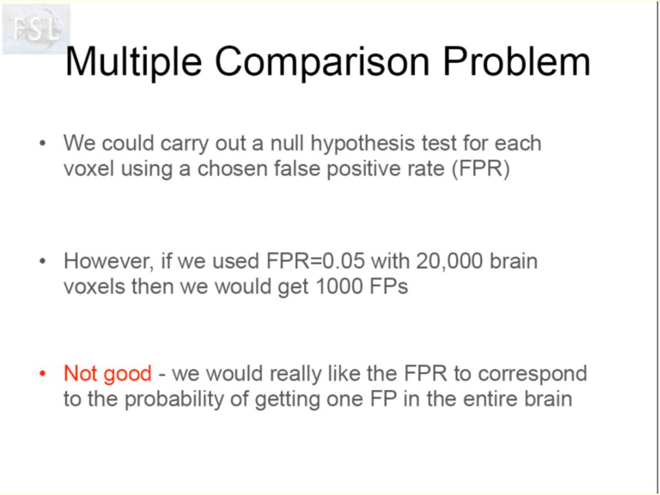


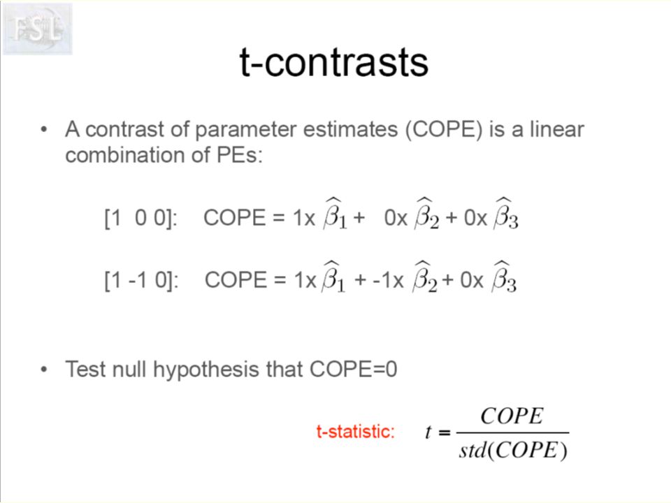

 forms a basis according to which.>")


 ● Standard Definitions ● Computing the DFT and FFT ● Sine and cosine wave multiplication.>")


>")
 Institute for Empirical.>")
