Download presentation
Presentation is loading. Please wait.

1
Using R to Model Complex Biogeochemical Systems
This talk is going to be a little bit different to most R User Group talks – instead of describing a new package, or some best practices, I’m just going to describe how R can be used as an alternative to traditional languages such as FORTRAN, to build mathematical models Chris Wood

2
Introduction to the science
Why are we interested in sediments? 71% of Earth’s surface (335,258,000 km2) Very dynamic environments Why are we interested in shelf-seas? Globally important sinks & sources for nutrients High rates of primary productivity Hello, I’m a PhD student from Southampton So, I know the vast majority of people here won’t be scientists, so will give a very quick overview of the science I’m looking at (I’ll keep it as simple as possible!), and then how I’ve used R to help me Diagenesis (what I study!) is the biochemical (bacterially-mediated) breakdown of organic matter in sediment So, why are we interested in sediments in general? Sediments are important! They probably contain every natural element (of which there are 94) Some sediments accumulate at more than 1 cm per year, and it can take just 11 days for material to sink from the top of the water column to the sediments which are 4000 metres deep. And, why specifically in shelf seas? The turquoise areas are shelf seas and continental shelf How PP changes in future. Sediments may supply 80% of nutrient demand of shelf phytoplankton BUT lack of knowledge of the magnitude of the sinks Primary production in shelf seas can be 10x higher than in the open ocean Although nutrient budgets for carbon and nitrogen have been estimated, and the flux from riverine and atmospheric sources are well quantified, sediments are less so, and that recycling of organic matter in sediment could be more important than previous budgets have accounted for 30% pp but 8% marine area Very shallow – the North Sea generally varies between just 30 and 100 m deep (i.e. less than 1% of the depth of the deep ocean!)
 Very dynamic environments. Why are we interested in shelf-seas Globally important sinks & sources for nutrients. High rates of primary productivity. Hello, I’m a PhD student from Southampton. So, I know the vast majority of people here won’t be scientists, so will give a very quick overview of the science I’m looking at (I’ll keep it as simple as possible!), and then how I’ve used R to help me. Diagenesis (what I study!) is the biochemical (bacterially-mediated) breakdown of organic matter in sediment. So, why are we interested in sediments in general Sediments are important! They probably contain every natural element (of which there are 94) Some sediments accumulate at more than 1 cm per year, and it can take just 11 days for material to sink from the top of the water column to the sediments which are 4000 metres deep. And, why specifically in shelf seas The turquoise areas are shelf seas and continental shelf. How PP changes in future. Sediments may supply 80% of nutrient demand of shelf phytoplankton BUT lack of knowledge of the magnitude of the sinks. Primary production in shelf seas can be 10x higher than in the open ocean. Although nutrient budgets for carbon and nitrogen have been estimated, and the flux from riverine and atmospheric sources are well quantified, sediments are less so, and that recycling of organic matter in sediment could be more important than previous budgets have accounted for. 30% pp but 8% marine area. Very shallow – the North Sea generally varies between just 30 and 100 m deep (i.e. less than 1% of the depth of the deep ocean!)")
3
Diagenesis results in fairly complicated set of feedback mechanisms and chemical profiles throughout the sediment column: For example: - oxygen breaks down organic matter – leading to this decrease in oxygen - ammonia is produced, this is oxidised by oxygen, producing nitrate (and also decreasing oxygen) - when oxygen runs out but there is still organic matter in the sediment, nitrate starts to break down the organic matter
 - when oxygen runs out but there is still organic matter in the sediment, nitrate starts to break down the organic matter.")
4
Main reactions Oxic zone – O2 mineralisation NO3- - denitrification
MnO2 reduction For those of you who don’t know much about sediment biogeochemistry, these are the basics. They’re all bacterially mediated Ammonia (not shown here) is a product of organic matter degradation Primary reactions of the oxidation of organic matter Zones of oxidation Waffle about MnO2 and NO3 being very close, and lack of MnO2 in most sediments BUT it is very localised – in some areas of the Skagerrak it is responsible for as much as 85% of organic matter oxidation – at 1 station sampled out of 11! All other stations were 0%! Hence not included in model SO42- isn’t on this diagram! Important! Other oxidants – iodate – have been suggested but few quantitative results Methanogenasis can occur in totally anoxic sediments (such as where OM flux is high enough to deplete all the oxidants here) Transport through the seidment is also important – advection, diffusion and bioturbation Fe(OH)3 reduction SO42- reduction Froelich et al. (1979)
 is a product of organic matter degradation. Primary reactions of the oxidation of organic matter. Zones of oxidation. Waffle about MnO2 and NO3 being very close, and lack of MnO2 in most sediments BUT it is very localised – in some areas of the Skagerrak it is responsible for as much as 85% of organic matter oxidation – at 1 station sampled out of 11! All other stations were 0%! Hence not included in model. SO42- isn’t on this diagram! Important! Other oxidants – iodate – have been suggested but few quantitative results. Methanogenasis can occur in totally anoxic sediments (such as where OM flux is high enough to deplete all the oxidants here) Transport through the seidment is also important – advection, diffusion and bioturbation. Fe(OH)3 reduction. SO42- reduction. Froelich et al. (1979)")
5
The maths… Despite the complexity, it can be described mathematically(!): Oxic breakdown of organic matter: Transport of chemical species Change in concentration of i Rate of consumption of i, but dependent on j It is known as the diagenetic equation Each chemical species, i, can be represented using this basic equation As shown on the previous slide, oxic breakdown is just one of the chemical reactions that makes up diageneis; this equation shows that there is a rate of organic matter breakdown, and that it is controlled by this Michaelis-Menten function that effectively controls that the breakdown doesn’t continue when all the oxygen has been consumed.

6
Transport ReacTran package
written for ecological and biogeochemical models; the examples in the vignette reflect this Grid <- setup.grid.1D(N=100,dx.1=0.1,L=15) Grid$x.mid, Grid$x.int, Grid$dx O2tran <- tran.1D (C=O2, C.up=bwO2, dx=Grid) Other arguments allow specific transport terms to be used As alluded to on the previous slide, all of the chemical species have some form of transport associated with them; all the transport happens within a grid pattern; ReacTran is a very generic package that can describe transport equations in 1, 2 or 3 dimensions; was written for ecological and biogeochemical models Exponential form (‘contains routines that enable the development of reactive transport models in aquatic systems (rivers, lakes, oceans), porous media (floc aggregates, sediments,...) and even idealized organisms (spherical cells, cylindrical worms,...)’) However… I don’t see any reason why any physical science problem that can be represented as happening in a grid, with associated fluxes between layers, couldn’t take advantage of the functions in this package So this 1 line of code calculates my grid for me, and returns a list containing (most usefully) 3 vectors; mid = position of middle of grid cells int = position of the interfaces of the grid cells dx = thickness of grid cells The transport of oxygen then returns a series of values, the most useful from a biogeochemical point of view is
 Grid$x.mid, Grid$x.int, Grid$dx. O2tran <- tran.1D (C=O2, C.up=bwO2, dx=Grid) Other arguments allow specific transport terms to be used. As alluded to on the previous slide, all of the chemical species have some form of transport associated with them; all the transport happens within a grid pattern; ReacTran is a very generic package that can describe transport equations in 1, 2 or 3 dimensions; was written for ecological and biogeochemical models. Exponential form. (‘contains routines that enable the development of reactive transport models in aquatic systems (rivers, lakes, oceans), porous media (floc aggregates, sediments,...) and even idealized organisms (spherical cells, cylindrical worms,...)’) However… I don’t see any reason why any physical science problem that can be represented as happening in a grid, with associated fluxes between layers, couldn’t take advantage of the functions in this package. So this 1 line of code calculates my grid for me, and returns a list containing (most usefully) 3 vectors; mid = position of middle of grid cells. int = position of the interfaces of the grid cells. dx = thickness of grid cells. The transport of oxygen then returns a series of values, the most useful from a biogeochemical point of view is.")
7
Solving the maths The deSolve and rootSolve packages
rootSolve: ‘Nonlinear root finding, equilibrium and steady-state analysis of ordinary differential equations’ deSolve: ‘General solvers for initial value problems of ordinary differential equations (ODE), partial differential equations (PDE), differential algebraic equations (DAE), and delay differential equations (DDE).’ Luckily, clever people have written some decent differential equation solvers as R packages – seemingly in a response to the lack of ode solvers that were available when they wrote their model: so, I use 2 packages that provide direct interfaces to the fortran and C functions. i.e. when I want to solve a steady-state (if no model parameters in the model are going to vary) solution to my model, I use methods from rootSolve; when I want to use solve a time-dependent solution to my model (for example, if I want to vary the organic matter input through an annual cycle, which is obviously more realistic), then I use deSolve methods
, partial differential equations (PDE), differential algebraic equations (DAE), and delay differential equations (DDE).’ Luckily, clever people have written some decent differential equation solvers as R packages – seemingly in a response to the lack of ode solvers that were available when they wrote their model: so, I use 2 packages that provide direct interfaces to the fortran and C functions. i.e. when I want to solve a steady-state (if no model parameters in the model are going to vary) solution to my model, I use methods from rootSolve; when I want to use solve a time-dependent solution to my model (for example, if I want to vary the organic matter input through an annual cycle, which is obviously more realistic), then I use deSolve methods.")
8
Solving the maths (cont…)
Simple to implement modelFunction <- function(t, y, pars){ #implementation of transport and differential #equations; e.g: OC <- y[1:100]; O2 <- y[101:200] oxicMin <- r*OC*(O2/(O2+ksO2oxic)) } ss.output <- steady.1D(y=rep(10,2*100), func=modelFunction, parms=c(r=10, ksO2oxic=1)) dyn.output <- ode.1D(y=ss.output$y, times=0:364, func=modelFunction, parms=pars) Solvers include RK4 etc etc… Simple to implement, even for a non-mathematician like me! 2 things to note – it is *much* quicker to solve the steady-state solution, and then use output from this as the argument to the dynamic solver – the vector y is of length number of layers by number of state variables, and (in this instance) gives the concentration of each of the state variables in each of the layers. Note that the only extra required argument in the dynamic solver is times – in this instance it’s in days Currently 13 solving methods (Runge-Kutta 4, euler, ode23 etc…) Output from dyn.output is a concentration per layer per time step All output from deSolve and rootSolve makes it very easy to create concentration profiles and contour plots
{ #implementation of transport and differential #equations; e.g: OC <- y[1:100]; O2 <- y[101:200] oxicMin <- r*OC*(O2/(O2+ksO2oxic)) } ss.output <- steady.1D(y=rep(10,2*100), func=modelFunction, parms=c(r=10, ksO2oxic=1)) dyn.output <- ode.1D(y=ss.output$y, times=0:364, func=modelFunction, parms=pars) Solvers include RK4 etc etc… Simple to implement, even for a non-mathematician like me! 2 things to note – it is *much* quicker to solve the steady-state solution, and then use output from this as the argument to the dynamic solver – the vector y is of length number of layers by number of state variables, and (in this instance) gives the concentration of each of the state variables in each of the layers. Note that the only extra required argument in the dynamic solver is times – in this instance it’s in days. Currently 13 solving methods (Runge-Kutta 4, euler, ode23 etc…) Output from dyn.output is a concentration per layer per time step. All output from deSolve and rootSolve makes it very easy to create concentration profiles and contour plots.")
9
Output The dynamic model run shows the results after a

10
Data management Data R + MySQL (+ RJDBC/rJava)
Multiple sites, cruises, repeat measurements & parameters R + MySQL (+ RJDBC/rJava) Post-processing / data consistency checking carried out in R Allows model calibration to be carried out I’m one of the lucky modellers who gets to help collect some data, so I spent a week on this research boat in the North Sea in September 2008 Modelling doesn’t just concern building a theoretical framework, it should represent real world data; Biogeochemical experiments can provide a lot of data; unfortunately, most analytical scientists don’t seem to have a particularly good grasp of data management… I’ve therefore done my own data management with the data I need to incorporate into the model Parameters here are measurements of nutrients and physical values; Quick example: nutrients typically measured at 1 cm resolution over cm – up to 8 nutrients at each site I used RJDBC and rJava as they seemed more stable and easier to setup than RMySQL So, I set up a simple relational database – this is an extract of the structure Data consistency is harder than it sounds! Perhaps as a result of the way I’m storing the data (which is very efficient to store, but not to check), my R code then has to check for multiple profiles, missing values etc
 Post-processing / data consistency checking carried out in R. Allows model calibration to be carried out. I’m one of the lucky modellers who gets to help collect some data, so I spent a week on this research boat in the North Sea in September Modelling doesn’t just concern building a theoretical framework, it should represent real world data; Biogeochemical experiments can provide a lot of data; unfortunately, most analytical scientists don’t seem to have a particularly good grasp of data management… I’ve therefore done my own data management with the data I need to incorporate into the model. Parameters here are measurements of nutrients and physical values; Quick example: nutrients typically measured at 1 cm resolution over cm – up to 8 nutrients at each site. I used RJDBC and rJava as they seemed more stable and easier to setup than RMySQL. So, I set up a simple relational database – this is an extract of the structure. Data consistency is harder than it sounds! Perhaps as a result of the way I’m storing the data (which is very efficient to store, but not to check), my R code then has to check for multiple profiles, missing values etc.")
11
Model testing & model calibration
Sensitivity analysis Allows us to discover the most sensitive model parameters Genetic algorithm (Relatively) efficient method of making model output fit real data There are many ways of carrying out sensitivity analysis – and there are methods in R packages (which I can talk about afterwards if people are interested), but I’ve written my own very simple ones GA – all I’m going to say is that it’s a way of making a model fit data – explaining it in detail would be a whole presentation in itself! The GA I’m using was (unfortunately) written in Matlab – but it is very simple to make Matlab run R code so that results from my model can be incorporated into the GA process at the appropriate times.
 efficient method of making model output fit real data. There are many ways of carrying out sensitivity analysis – and there are methods in R packages (which I can talk about afterwards if people are interested), but I’ve written my own very simple ones. GA – all I’m going to say is that it’s a way of making a model fit data – explaining it in detail would be a whole presentation in itself! The GA I’m using was (unfortunately) written in Matlab – but it is very simple to make Matlab run R code so that results from my model can be incorporated into the GA process at the appropriate times.")
12
Future ideas / personal interests
Web-based model-runs via R + python (mod_python / rpy2) R would provide better graphics than currently available via PHP libraries Greater access for non-modeller researchers Public engagement of science These aren’t really within the boundaries of my PhD, but they’re ideas I’d be interested in seeing implemented in the future unfortunately, rpy2 doesn’t seem stable on windows with recent versions of R In my brief experience, even where models are implemented within frameworks, some researchers who want to use (not develop) a model are put off by having to deal with any kind of code – running models through a web-interface would eliminate this problem With simple models that had public interest (such as climate change or ocean acidication!), would be easy for a public engagement / educational project to allow users to a website to see the effect of the changes of 1 or 2 input parameters on model output
 R would provide better graphics than currently available via PHP libraries. Greater access for non-modeller researchers. Public engagement of science. These aren’t really within the boundaries of my PhD, but they’re ideas I’d be interested in seeing implemented in the future unfortunately, rpy2 doesn’t seem stable on windows with recent versions of R. In my brief experience, even where models are implemented within frameworks, some researchers who want to use (not develop) a model are put off by having to deal with any kind of code – running models through a web-interface would eliminate this problem. With simple models that had public interest (such as climate change or ocean acidication!), would be easy for a public engagement / educational project to allow users to a website to see the effect of the changes of 1 or 2 input parameters on model output.")
13
Any questions? Acknowledgements: Funding: NERC & Defra
University of Southampton Boris Kelly-Gerreyn, Peter Statham, Adrian Martin, Andy Yool, John Hemmings, Charlie Thompson, Carl Amos Netherlands Institute of Ecology Karline Soetaert, Filip Meysman University of Portsmouth Gary Fones, Fay Couceiro, Adam Hamilton Cefas John Aldridge, Ruth Parker, Dave Sivyer, Johan van Molen, Naomi Greenwood, Elke Neubacher UEA Keith Weston Partrac Ltd Kevin Black, Rachel Helsby Crew of Cefas Endeavour Main aims Objectives The importance Initial considerations Multidisciplinary approach Our model Current results Observations Conclusions

14
The importance of nutrients in the coastal ocean
Shelf seas: Globally important sinks & sources for nutrients High rates of primary productivity Knowledge of nutrient origin & fate is key to understanding primary productivity Sediments are potentially important sources of nutrients in shelf seas Need to be able to model sediment systems to predict nutrient exchanges How PP changes in future. Sediments may supply 80% of nutrient demand of shelf phytoplankton BUT lack of knowledge of the magnitude of the sinks 30% pp but 8% marine area Hence understanding nutrient fate after resuspension events could affect our thinking of how the ecosystem works – including all the way up the food chain Primary production in shelf seas can be 10x higher than in the open ocean Although nutrient budgets for carbon and n itrogen have been estimated, and the flux from riverine and atmospheric sources are well quantified, sediments are less so, and that recycling of organic matter in sediment could be more important than previous budgets have accounted for Where ED is The physical, biological & chemical changes which occur to deposited material during burial in sediment Oxidation of organic matter and reoxidation of reduced species Transport (advection, diffusion & bioturbation) Leads to hypothesis that the sediments are a source of nutrients
 Leads to hypothesis that the sediments are a source of nutrients.")
15
Results from genetic algorithm
Mention which profile is which! Should be noted that this process was iterative – running the GA, seeing results (both graphically and quantitatively), and adjusting the ranges - for example, here’s a set which didn’t work very well! - note that O2 is fairly good, but nitrate shows too great a peak and goes down to zero whereas expt doesn’t – (ie in experiments, only oxic mineralisation and denitrification occur, whereas model output would imply that more mineralisation reactions occur) - carbon and ammonia are a long way out!
, and adjusting the ranges. - for example, here’s a set which didn’t work very well! - note that O2 is fairly good, but nitrate shows too great a peak and goes down to zero whereas expt doesn’t – (ie in experiments, only oxic mineralisation and denitrification occur, whereas model output would imply that more mineralisation reactions occur) - carbon and ammonia are a long way out!")
16
Results from genetic algorithm

17
Analysis of genetic algorithm output
Are values sensible? Parameter OMEXDIA value GA result Mean flux (g C m-2 yr-1) - 16 Bioturbation (cm2 d-1) 1/365 17/365 rFast (d-1) 0.01 0.0576 rSlow (d-1) 0.0001 pFast 0.9 0.9515 NCrFdet (mol N : mol C) 0.16 Are the values sensible? Although we used relatively constrained ranges, it’s still worth checking all the parameters to make sure that they all seem sensible. Obviously won’t show all param values here – too many, but the significant ones are: Mean Flux (forcing parameter) – seemed to act sensibly in range of 1-50 g C m2 yr-1 Note that NCrFdet is same – others aren’t too different. Increase in biot not a surprise; majority of North Sea has high biological turnover (17/365 is ~0.05) - This is still at the lower end of bioturbation in coastal sediments – literature values go up to 1 cm2 d-1
 Bioturbation (cm2 d-1) 1/ /365. rFast (d-1) rSlow (d-1) pFast NCrFdet (mol N : mol C) Are the values sensible Although we used relatively constrained ranges, it’s still worth checking all the parameters to make sure that they all seem sensible. Obviously won’t show all param values here – too many, but the significant ones are: Mean Flux (forcing parameter) – seemed to act sensibly in range of 1-50 g C m2 yr-1. Note that NCrFdet is same – others aren’t too different. Increase in biot not a surprise; majority of North Sea has high biological turnover (17/365 is ~0.05) - This is still at the lower end of bioturbation in coastal sediments – literature values go up to 1 cm2 d-1.")
18
Evaluation of outputs Are all processes well explained by model?
How important is the benthic fluff layer? Do more mineralisation reactions need to be included in the model? Should other biogeochemical processes be included? Has model been ‘over-fitted’? Processes - Fluff layer? Fluff layers would show that there is high levels of mineralisation of OM in the water. This would distort the organic carbon flux to the sediment, and might also distort the associated parameters, such as pFast (ratio of fast degrading organic matter) and nitrogen:carbon ratios. Characterisation of the fluff material is very difficult, and (as far as I know), nobody has been able to give any quantitative indication of mineralisation rates Other mineralisation reactions: as stated, model only has oxic mineralisation and dentrification included; although manganese oxide reduction is unlikely to be an important process, sulphate reduction may be important in some localised areas – some studies have found that sulphate reduction could be responsible for upto 80% of OM mineralisation in some areas of the North Sea. If there are very high rates of bioturbation (which is likely), then significant mixing of the sediment will occur – this could mean that although the nitrate profiles indicate (under traditional thinking) that no further mineralisation occurs, it is possible that the denitrification and sulphate reduction processes overlap significantly – this would be difficult to model. Other biogeochemical processes – such as anammox (ANaerobic AMMonium Oxidation) – have been shown to occur in coastal sediments. Over-fitted – i.e. have we allowed too much freedom in the parameters? However – the parameter values from the original OMEXDia model are for slope, not shelf, so would expect different values for virtually all parameters
 and nitrogen:carbon ratios. Characterisation of the fluff material is very difficult, and (as far as I know), nobody has been able to give any quantitative indication of mineralisation rates. Other mineralisation reactions: as stated, model only has oxic mineralisation and dentrification included; although manganese oxide reduction is unlikely to be an important process, sulphate reduction may be important in some localised areas – some studies have found that sulphate reduction could be responsible for upto 80% of OM mineralisation in some areas of the North Sea. If there are very high rates of bioturbation (which is likely), then significant mixing of the sediment will occur – this could mean that although the nitrate profiles indicate (under traditional thinking) that no further mineralisation occurs, it is possible that the denitrification and sulphate reduction processes overlap significantly – this would be difficult to model. Other biogeochemical processes – such as anammox (ANaerobic AMMonium Oxidation) – have been shown to occur in coastal sediments. Over-fitted – i.e. have we allowed too much freedom in the parameters However – the parameter values from the original OMEXDia model are for slope, not shelf, so would expect different values for virtually all parameters.")
19
Conclusions & future work
The GA is able to give a good fit with sensible parameter values, but: How much predictive ability does this model have? Effect of increasing number of biogeochemical processes? Incorporate a simple sediment resuspension model into current model The model could help in calculating nutrient budgets of shelf seas? So, basically this work shows only 1 conclusion! Especially with regard to bioturbation, although a bioturbation coefficient could never account for individual worm holes For example – estimate values for organic matter flux to the sediment, ratios of fast, slow and refractory carbon Would a more complex model help or hinder using the model for predictive ability? Biogeochemical processes to include mineralisation routes and other biogeochemical processes - anammox (and making others more complex – e.g. introducing Q10 – this could be more of a consideration in coastal seas than continental slopes / deep sea) Nutrient budget of shelf-seas is ultimate goal in biogeochemical modelling
 Nutrient budget of shelf-seas is ultimate goal in biogeochemical modelling.")
20
Sensitivity analysis 3 simple sensitivity analysis experiments were carried out – each with an upper and lower value: Literature data Double and halve the default values Order of magnitude above and below the default value Non-linearity of model leads to unexpected results A sensitivity analysis allows us to determine which parameters in the model have the greatest effect on the model outcome The model is run using the upper and lower values, changing each parameter in turn and leaving the rest as default values; i.e. for these 3 sets of upper and lower values with 26 parameters, I’m running the model 3*2*26 times = 156 Unexpected results such as doubling and halving the same parameter lead to vastly different effects on model

21
Sensitivity analysis results
Purposefully not put all graphs here – they are difficult to interpret and have a lot of data in a small amount of space! Cost function is effectively just a root mean square away from default model output This is just an example of the magnitudes of the cost functions, and how different they can be – this graph is log of the cost function We have decided from the results to use the following 6 - explain what the parameters are! Note that there is no bioirrigation in the model – how to and whether you should distinguish between sediment transport and interstitial porewater transport still seems to be a contentious issue in the literature! Note also other methods – Latin Hypercube etc. However, the method we have chosen is the most common method to use *and* produces results that match previous work as well as producing results that seem the most sensible from a biogeochemical point of view

22
Observational data POINT OUT O2 SCALE!
This is the raw data from the Oyster Grounds – unfortuantely not as much nitrate and ammonia data as we’d like TOC seems to imply that it the fastest degrading carbon is consumed at the surface of the sediment, or even in the water column, and that what is left is the refractory content O2 penetrtation slighly deeper in feb – what you’d expect before the spring bloom Nitrate shows slight peak – nitrification before decrease due to denitrification – although the resolution isnt very high NH3 shows increase as we’d expect

23
Comparison with observations
After sensitivity analysis of the full parameter set had been carried out, 3 parameters were modified in the steady-state model These graphs show a range of POC fluxes which is the main forcing parameter in the model Is able to give a fairly good representation of the TOC Not very good O2 NO3 is fairly hard to judge because of low resolution, but it seems that the model over estimates nitrification at the moment NH3 isnt bad but might be overestimating production Data implies that no degradable carbon after ~ 5 cm because of NO3 and NH3 data However – data has problems – heterogeneity – no 2 places will be the same and the same site will also be changing – difficult to determine which data to use to best fit a model Dogger Bank – also slighly muddy sediment, shows same trends and so isnt shown

24
Sensitivity analysis results
Increased cost function implies more sensitive parameter Ranking all results into a single list allows us to pick an arbitrary number of parameters to use in future experiments Mean Flux NCrFdet pFast rSlow rFast biot Purposefully not put all graphs here – they are difficult to interpret and have a lot of data in a small amount of space! Cost function is effectively just a root mean square away from default model output This is just an example of the magnitudes of the cost functions, and how different they can be – this graph is log of the cost function We have decided from the results to use the following 6 - explain what the parameters are! Note that there is no bioirrigation in the model – how to and whether you should distinguish between sediment transport and interstitial porewater transport still seems to be a contentious issue in the literature! Note also other methods – Latin Hypercube etc. However, the method we have chosen is the most common method to use *and* produces results that match previous work as well as producing results that seem the most sensible from a biogeochemical point of view

25
Optimising model to data: Genetic Algorithm
The population is the set of free parameters A generation is a set of model runs equal to the number of free parameters Initial run: randomly generated parameter set from a range given to the algorithm Parameter values are converted into binary to allow ‘genetic crossover’ between random pairs of parameters Subsequent runs: The model is run for n generations * m unconstrained parameters 5000 * 30 = (~28 hrs) Parents: Crossover point We have a task of being able to fit model output to observational data; although we can manually modify the parameters in order to improve the fit, this model (which, as already mentioned, is relatively complicated) has 26 parameters – only 4 can be constrained by experimental data: bwO2, bwNH3, bwNH3, C:N ratio (although, OMEXDia models fast degrading and slow degrading carbon separately – this can’t be resolved experimentally – talk about later); the other 25 can only be given ranges which we hope are sensible. This leads onto the method we’ve used – a genetic algorithm - params that aren’t constrained – in this model, so little understood that all parameters included. for expt data - ranges given to model: unconstrained params – very wide ranges (typically an order of magnitude either side of values given in original omexdia model) – expt data – range is range of all data (not segregated by season or site) - Each new generation uses values from the previous generation Children:
 Parents: Crossover point. We have a task of being able to fit model output to observational data; although we can manually modify the parameters in order to improve the fit, this model (which, as already mentioned, is relatively complicated) has 26 parameters – only 4 can be constrained by experimental data: bwO2, bwNH3, bwNH3, C:N ratio (although, OMEXDia models fast degrading and slow degrading carbon separately – this can’t be resolved experimentally – talk about later); the other 25 can only be given ranges which we hope are sensible. This leads onto the method we’ve used – a genetic algorithm. - params that aren’t constrained – in this model, so little understood that all parameters included. for expt data. - ranges given to model: unconstrained params – very wide ranges (typically an order of magnitude either side of values given in original omexdia model) – expt data – range is range of all data (not segregated by season or site) - Each new generation uses values from the previous generation. Children:")
26
Example of inhibition

27
Current understanding of early diagenesis
Euphotic zone PP = 250 g C m-2 yr-1 (1) 370 g C m-2 yr-1 (2) Thermocline has little effect, although cells sink out… with a short delay at the pycnocline (1) Fluxes: Corg: 50-90% recycled [1) Corg: 2 µmol cm-2 d-1 [2] NO2- + NO3-: -160 – 309 µmol m-2 d-1 (5, 6) NH4+: -400 – 66 µmol m-2 d-1 (5, 6) PO4: µmol m-2 d-1 (16) 1.1 5.2 ΣCO2 (g d.w.)-1 d-1 Fe2+ flux increases (7 – 22 [modelled] / 46 [in situ measurement] nmol cm-2 d-1) as O2 of BW decreases (300 -> 0 µM) [6] 10-50% (1, 2) ‘Normal’: ~340 mg Spring bloom: 185 mg C m-2 d-1 (12-21%) (3) Si(OH)3 – 0.05 – 0.2 µmol cm-2 d-1 [6] Sediment-water interface (SWI) Corg metabolism: 12 – 23 mmol C cm-2 day-1 (4) Shelf sea Corg content = 1-5% Brockmann et al. (1990) Wollast (1991) Kuhn & Radach (1997) Billen et al. (1990) van Raaphorst et al. (1990) Hall et al. (1996) van der Weijden (1992) Fang et al. (2007) Canfield et al. (1993) Wijsmann et al. (2002) Ussher et al. (2007) Overnell (2002) Rysgaard et al. (2001) Price et al. (1994) Jorgensen (1977) Slomp et al. (1998) Z Diagenesis is series of reactions describing reactions in sediment – early diagenesis = fate of SPM – top few cms Thermocline – 30m (2) Kuhn & Radach (1997) Total Corg metabolism = 140 – 280 mg C m-2 d-1 (12-23 mmol C m-2 d-1) Bacterial counts / biomass not very accurate: biomass estimates in North Sea range from 1 x 10⁻⁴ to 1 x 10⁻³ mg C g. Counts 108 – 1010 cm-2 Recycled = grazing / remineralisation Buried: 1% of pp - Total for N Sea = 2 x10⁶ tons [~1(6) – 4 (3) g m-2 yr-1] Carbon higher in shelf sea sediments than slopes (2%) and deep sea sediments (0.3%) Carbon flux out of sediments ~= > 40% of PP is flux out of sediment: 2 µmol cm-2 d-1 Penetration depth: upto 1 cm in summer / following spring-bloom (but Lohse et al. (1996) very high oxidation can mean that oxygen penetration is negative - ~-250 µm – result of reduced compounds released from sediment into water column NH4 + O2 NO3) – deeper penetration in winter [up to 45 mm] (no oxidation of OM) OXYGEN Oxygen consumption: 1 (Weston et al., 2008 – Dogger Bank, 35 – 50 m, late summer 2003) – 3 (Nakamura, 2003 – Seto Inland Sea, summer 2000) mmol m-2 hr-1 Relative Corg oxidation by O2? NITROGEN Hall et al: Skagerrak Brockmann et al. North Sea - winter and spring Nitrate + nitrite can be up to 50 µmol in coastal zones in winter Surface waters: in general, minima during spring bloom, highest in winter, but also: during the winter cruise, nutrient minima were detected in the Dogger Bank area. This is an indication that primary production continues during winter Bottom waters: ammonium: 0.5 (winter) – 3 (summer) µmol l-1 Brockmann et al. (1990): near bottom waters, nitrite + nitrate can be [spring bloom] 0.1 (mixed waters) 3-6 (stratified waters) µmol l-1 Ammonium up to 10 µmol in coastal zones in winter. High NH4+ in open water shows remineralisation Nitrite + nitrate near bottom waters: Ammonium: higher values in summer show mineralisation Mixed – 0.1 – 1 µmol [BUT can be up to 6 sometimes – shows that there is oxidation of mineralised organic matter] Stratified – 3-6 µmol – even up to 50 in some coastal zones Observational evidence of net gain of nitrate, nitrite and ammonium by sediment Fluxes of nitrogen species: Ammonium flux shows, in general, a trend throughout the year that there is a flux out of the sediment early in the year, then during and post bloom, the flux is into the sediment (of course! – degradation of OM) Hall et al. (1996) determined nitrite and nitrate separately, which showed that nitrate was much higher concs, but also more variable (-140 – 300); nitrite was -20 – 4.7. Little difference between stratified and mixed waters of nitrate / nitrite flux NO3 (+ NO2) flux shows flux out of sediment in March and August/ September, but in general, a flux into the sediment in May [oxidised OM settling] - higher values result of oxidation of mineralised organic matter van Raaphorst et al. was done in Dogger Bank so may be slightly more relevant – July / Aug 1988 Hall (the later study) showed less variation in ammonium (-61 – 45; earlier showed -400 – 66) Nitrate consumption: Note units (mmol – as opposed to nmol for other oxidants – i.e. relatively important) – equivalent C units: 4.6 mmol C m-2 d-1 (i.e. up to 1/3) In O2 reduction zone (i.e. oxic zone), NO3 conc increases (oxidation of degraded organic matter) - nitrification [NO3-] decreases Below oxic zone (marked by (d2[NO3-])/dz2 = 0), denitrification and NO3 reduction rate exceeds oxidation: Phosphate: little differences between mixed and stratified water Surface waters: 0.1 – 2 µmol l-1 (Brockmann et al. (1990)) lower concs in spring bloom Bottom water concs similar to surface waters – mixed 0.1 (all taken up – recycled faster than mineralisation) – stratified & winter – 2 Flux: Very small flux in to water column in summer (except in 1 location which was ~10x higher), virtually no flux (nanomolr concs) during winter Fe-bound P is ~8% so could also be a significant sink CFA burial: 5.8% = proportion of total phosphorous pool lost to sediment IRON Biota uptake very important: 40 µmol Fe (g Chl a)-1 h-1 Very low concs in surface waters (0.6 nmol l-1 on European shelf) [11 – Ussher et al (2007)] Fe3+ contributes up to 78% of C oxidation in anoxic coastal sediments [Canfield et al. (1993)] Carbon oxidation rates (113 – 401 / nmole cm-2 d-1] significantly increase below oxic zone Fluxes: flume experiments have also been done which show (again) slight differences: nmol cm-2 d-1 [Huettel et al. (1998)] Biota uptake rates was in summer 1990 in open Pacific Ocean [Price et al (1994)] Rysgaard et al. (2001) – Skaggerak & Kattegat. Highest rate is at 43 m / 56 m is 560 / 200 m is 500 / 25 m is 60 – 130 (2 sites) Overnell – [20 – 300 nmol cm-2 d-1] Scottish Loch [water depth: 75 – 145 m] modelled results based on Slomp et al. (1997) / collected in Nov 1996 – Feb 1997 (will have lower rates anyway) This explains the rapid increase in Fe2+ conc in suboxic zone, until rapid removal when FeS is produced (SO42- is lower oxidiser, therefore lower) in summer (no major increase in winter) Fe(III) and S(VI) reduction give Fe2+ + S2- FeS + H2S pyrite Contributes up to 76% in Kattegat (Rysgaard et al. (2001)) MANGANESE In theory, same order of magnitude importance as Fe (up to 2 orders less important than O2). MnO2 profile is very similar to SO42- [and Fe3+] – 30 µM at surface 0 by 10 cm in tidal areas (Dellwig et al. (2007)) – enhanced microbial activity leads to increase in Mn oxides reduction, and enhance Mn2+ flux BUT In open waters, there few reducable Mn forms (conversly, Fe is found as Fe crystals), so it actually does not contribute much to the Corg oxidation (Rysgaard et al, 2001) SULPHUR Sulphate reduction is 50 in winter and up to 400 in summer Sulphate reduction causes 220 mg C m-2 d-1 (where O2 penetration is < 10mm) – 18 mmol C m-2 d-1 As sulphate is reduced, concs of other species of sulphur (sulphide and thiosulphate – S2O32-) increase; sulphide then reduces as FeS / FeS2 are formed Virtually no flux (4-7 orders of magnitude lower than nitrogen species and oxygen - < 20 picomol cm-2 d-1) Pyrite: at z = 2 cm, FeS2 = 30 µmol g-1, increases to 150 at z = 50 SILICATE Silicate cycling is more simple than other elements – silicate fluxes show relatively little difference (majority are between 1 and 2 nmol cm-2 d-1) – biogenic silica = shells of diatoms – taken up in water column. Silicon in water column: surface waters: 0.5 – 2 µmol l-1 (summer) – taken up by diatoms / up to 30 µmol l-1 in winter Bottom waters reflect surface waters when mixed - stratified waters: Si(OH)3 concs lower in spring than in winter by up to 2.5 µmol l-1 [slow mineralisation wrt other nutrients] RESUSPENSION Nutrients seem to be affected – e.g. increased nitrification / denitrification (Dale & Prego, 2002 – North-West Spain coast); resuspension can be a source of Fe concentrations in North Sea [3 nmol l-1] (Nedelec et al, 2007); short resuspension events (5 seconds every 24 hrs) can increase mineralisation rates of OM from 1.1 to 5.2 ΣCO2 (g d.w.)-1 d-1 (even greater than continuous resuspension) – however, shear stress wasn’t considered – perhaps very low shear stress would promote mineralisation, and then resuspension would not cause any additional enhancement [Stahlberg et al., 2006] Not much work done specifically in North Sea Lee et al. (PROWQM model) modelled the resuspension, but not the affect on concentrations Jones et al. (1998) (obs paper) found that resuspension caused greater proportion of OM remineralisation in water column rather than benthic (but didn’t give values) Continental shelves have been shown to be a source of trace metals (Southern Ocean) – dFe at bed (80 m) = 15 nM, 10 nM at 50 m (Bucciarelli et al. (2001)) North-east Irish Sea: difficult to quantify (Williams et al, 1998) Fe3+ reduction rates: (12) / (13) nmol cm-2 d-1 Nitrate reduction: 0.7 mmol m-2 d-1 (7) Z < 1 cm: 113 – 401 nmole cm-2 d-1 [9] 1 < Z (cm) < 4: 387 – 1987 nmole cm-2 d-1 [9] Corg metabolism: 18 mmol C m-2 d-1 (9) SO42- reduction: nmol cm-3 d-1 (15) Z Permanently buried: Corg ~1% (2) CFA: 5.8 % (8) Pyrite formation: 8.9 x10⁻⁶ µmol l-1 d-1 (10)
 370 g C m-2 yr-1 (2) Thermocline has little effect, although cells sink out… with a short delay at the pycnocline (1) Fluxes: Corg: 50-90% recycled [1) Corg: 2 µmol cm-2 d-1 [2] NO2- + NO3-: -160 – 309 µmol m-2 d-1 (5, 6) NH4+: -400 – 66 µmol m-2 d-1 (5, 6) PO4: µmol m-2 d-1 (16) 1.1 5.2 ΣCO2 (g d.w.)-1 d-1. Fe2+ flux increases (7 – 22 [modelled] / 46 [in situ measurement] nmol cm-2 d-1) as O2 of BW decreases (300 -> 0 µM) [6] 10-50% (1, 2) ‘Normal’: ~340 mg. Spring bloom: 185 mg C m-2 d-1 (12-21%) (3) Si(OH)3 – 0.05 – 0.2 µmol cm-2 d-1 [6] Sediment-water interface (SWI) Corg metabolism: 12 – 23 mmol C cm-2 day-1 (4) Shelf sea Corg content = 1-5% Brockmann et al. (1990) Wollast (1991) Kuhn & Radach (1997) Billen et al. (1990) van Raaphorst et al. (1990) Hall et al. (1996) van der Weijden (1992) Fang et al. (2007) Canfield et al. (1993) Wijsmann et al. (2002) Ussher et al. (2007) Overnell (2002) Rysgaard et al. (2001) Price et al. (1994) Jorgensen (1977) Slomp et al. (1998) Z. Diagenesis is series of reactions describing reactions in sediment – early diagenesis = fate of SPM – top few cms. Thermocline – 30m (2) Kuhn & Radach (1997) Total Corg metabolism = 140 – 280 mg C m-2 d-1 (12-23 mmol C m-2 d-1) Bacterial counts / biomass not very accurate: biomass estimates in North Sea range from 1 x 10⁻⁴ to 1 x 10⁻³ mg C g. Counts 108 – 1010 cm-2. Recycled = grazing / remineralisation. Buried: 1% of pp - Total for N Sea = 2 x10⁶ tons [~1(6) – 4 (3) g m-2 yr-1] Carbon higher in shelf sea sediments than slopes (2%) and deep sea sediments (0.3%) Carbon flux out of sediments ~= > 40% of PP is flux out of sediment: 2 µmol cm-2 d-1. Penetration depth: upto 1 cm in summer / following spring-bloom (but Lohse et al. (1996) very high oxidation can mean that oxygen penetration is negative - ~-250 µm – result of reduced compounds released from sediment into water column NH4 + O2 NO3) – deeper penetration in winter [up to 45 mm] (no oxidation of OM) OXYGEN. Oxygen consumption: 1 (Weston et al., 2008 – Dogger Bank, 35 – 50 m, late summer 2003) – 3 (Nakamura, 2003 – Seto Inland Sea, summer 2000) mmol m-2 hr-1. Relative Corg oxidation by O2 NITROGEN. Hall et al: Skagerrak. Brockmann et al. North Sea - winter and spring. Nitrate + nitrite can be up to 50 µmol in coastal zones in winter. Surface waters: in general, minima during spring bloom, highest in winter, but also: during the winter cruise, nutrient minima were detected in the Dogger Bank area. This is an indication that primary production continues during winter. Bottom waters: ammonium: 0.5 (winter) – 3 (summer) µmol l-1. Brockmann et al. (1990): near bottom waters, nitrite + nitrate can be [spring bloom] 0.1 (mixed waters) 3-6 (stratified waters) µmol l-1. Ammonium up to 10 µmol in coastal zones in winter. High NH4+ in open water shows remineralisation. Nitrite + nitrate near bottom waters: Ammonium: higher values in summer show mineralisation. Mixed – 0.1 – 1 µmol [BUT can be up to 6 sometimes – shows that there is oxidation of mineralised organic matter] Stratified – 3-6 µmol – even up to 50 in some coastal zones. Observational evidence of net gain of nitrate, nitrite and ammonium by sediment. Fluxes of nitrogen species: Ammonium flux shows, in general, a trend throughout the year that there is a flux out of the sediment early in the year, then during and post bloom, the flux is into the sediment (of course! – degradation of OM) Hall et al. (1996) determined nitrite and nitrate separately, which showed that nitrate was much higher concs, but also more variable (-140 – 300); nitrite was -20 – 4.7. Little difference between stratified and mixed waters of nitrate / nitrite flux. NO3 (+ NO2) flux shows flux out of sediment in March and August/ September, but in general, a flux into the sediment in May [oxidised OM settling] - higher values result of oxidation of mineralised organic matter. van Raaphorst et al. was done in Dogger Bank so may be slightly more relevant – July / Aug Hall (the later study) showed less variation in ammonium (-61 – 45; earlier showed -400 – 66) Nitrate consumption: Note units (mmol – as opposed to nmol for other oxidants – i.e. relatively important) – equivalent C units: 4.6 mmol C m-2 d-1 (i.e. up to 1/3) In O2 reduction zone (i.e. oxic zone), NO3 conc increases (oxidation of degraded organic matter) - nitrification. [NO3-] decreases. Below oxic zone (marked by (d2[NO3-])/dz2 = 0), denitrification and NO3 reduction rate exceeds oxidation: Phosphate: little differences between mixed and stratified water. Surface waters: 0.1 – 2 µmol l-1 (Brockmann et al. (1990)) lower concs in spring bloom. Bottom water concs similar to surface waters – mixed 0.1 (all taken up – recycled faster than mineralisation) – stratified & winter – 2. Flux: Very small flux in to water column in summer (except in 1 location which was ~10x higher), virtually no flux (nanomolr concs) during winter. Fe-bound P is ~8% so could also be a significant sink. CFA burial: 5.8% = proportion of total phosphorous pool lost to sediment. IRON. Biota uptake very important: 40 µmol Fe (g Chl a)-1 h-1. Very low concs in surface waters (0.6 nmol l-1 on European shelf) [11 – Ussher et al (2007)] Fe3+ contributes up to 78% of C oxidation in anoxic coastal sediments [Canfield et al. (1993)] Carbon oxidation rates (113 – 401 / nmole cm-2 d-1] significantly increase below oxic zone. Fluxes: flume experiments have also been done which show (again) slight differences: nmol cm-2 d-1 [Huettel et al. (1998)] Biota uptake rates was in summer 1990 in open Pacific Ocean [Price et al (1994)] Rysgaard et al. (2001) – Skaggerak & Kattegat. Highest rate is at 43 m / 56 m is 560 / 200 m is 500 / 25 m is 60 – 130 (2 sites) Overnell – [20 – 300 nmol cm-2 d-1] Scottish Loch [water depth: 75 – 145 m] modelled results based on Slomp et al. (1997) / collected in Nov 1996 – Feb 1997 (will have lower rates anyway) This explains the rapid increase in Fe2+ conc in suboxic zone, until rapid removal when FeS is produced (SO42- is lower oxidiser, therefore lower) in summer (no major increase in winter) Fe(III) and S(VI) reduction give Fe2+ + S2- FeS + H2S pyrite. Contributes up to 76% in Kattegat (Rysgaard et al. (2001)) MANGANESE. In theory, same order of magnitude importance as Fe (up to 2 orders less important than O2). MnO2 profile is very similar to SO42- [and Fe3+] – 30 µM at surface 0 by 10 cm in tidal areas (Dellwig et al. (2007)) – enhanced microbial activity leads to increase in Mn oxides reduction, and enhance Mn2+ flux. BUT. In open waters, there few reducable Mn forms (conversly, Fe is found as Fe crystals), so it actually does not contribute much to the Corg oxidation (Rysgaard et al, 2001) SULPHUR. Sulphate reduction is 50 in winter and up to 400 in summer. Sulphate reduction causes 220 mg C m-2 d-1 (where O2 penetration is < 10mm) – 18 mmol C m-2 d-1. As sulphate is reduced, concs of other species of sulphur (sulphide and thiosulphate – S2O32-) increase; sulphide then reduces as FeS / FeS2 are formed. Virtually no flux (4-7 orders of magnitude lower than nitrogen species and oxygen - < 20 picomol cm-2 d-1) Pyrite: at z = 2 cm, FeS2 = 30 µmol g-1, increases to 150 at z = 50. SILICATE. Silicate cycling is more simple than other elements – silicate fluxes show relatively little difference (majority are between 1 and 2 nmol cm-2 d-1) – biogenic silica = shells of diatoms – taken up in water column. Silicon in water column: surface waters: 0.5 – 2 µmol l-1 (summer) – taken up by diatoms / up to 30 µmol l-1 in winter. Bottom waters reflect surface waters when mixed - stratified waters: Si(OH)3 concs lower in spring than in winter by up to 2.5 µmol l-1 [slow mineralisation wrt other nutrients] RESUSPENSION. Nutrients seem to be affected – e.g. increased nitrification / denitrification (Dale & Prego, 2002 – North-West Spain coast); resuspension can be a source of Fe concentrations in North Sea [3 nmol l-1] (Nedelec et al, 2007); short resuspension events (5 seconds every 24 hrs) can increase mineralisation rates of OM from 1.1 to 5.2 ΣCO2 (g d.w.)-1 d-1 (even greater than continuous resuspension) – however, shear stress wasn’t considered – perhaps very low shear stress would promote mineralisation, and then resuspension would not cause any additional enhancement [Stahlberg et al., 2006] Not much work done specifically in North Sea. Lee et al. (PROWQM model) modelled the resuspension, but not the affect on concentrations. Jones et al. (1998) (obs paper) found that resuspension caused greater proportion of OM remineralisation in water column rather than benthic (but didn’t give values) Continental shelves have been shown to be a source of trace metals (Southern Ocean) – dFe at bed (80 m) = 15 nM, 10 nM at 50 m (Bucciarelli et al. (2001)) North-east Irish Sea: difficult to quantify (Williams et al, 1998) Fe3+ reduction rates: (12) / (13) nmol cm-2 d-1. Nitrate reduction: 0.7 mmol m-2 d-1 (7) Z < 1 cm: 113 – 401 nmole cm-2 d-1 [9] 1 < Z (cm) < 4: 387 – 1987 nmole cm-2 d-1 [9] Corg metabolism: 18 mmol C m-2 d-1 (9) SO42- reduction: nmol cm-3 d-1 (15) Z. Permanently buried: Corg ~1% (2) CFA: 5.8 % (8) Pyrite formation: 8.9 x10⁻⁶ µmol l-1 d-1 (10)")
28
Multidisciplinary approach
NOCS, University of Portsmouth, CEFAS & Partrac Ltd A project of the Marine Ecosystems Connection – NERC and Defra funded & organised by Cefas Multi disciplinary approach leads to greater understanding by being able to link different processes together Combined modelling, observational & experimental approach Dogger Bank transect deg N, ~1 deg E

29
Why include resuspension?
Previous work has concentrated on other sources of nutrients Frequent resuspension events Release of nutrients Sink for nutrients Resuspension may be involved in regulating primary production Previous work: atmospheric, riverine, diffusive and boundary fluxes considered, but not resuspension Regulate primary productivity BUT we don’t know to what extent North Sea is only 30 m deep in some places – this means that tides, currents and storms can impact the sediment As sediment is resuspended, ability to release organic matter trapped in the layers amount resuspended could be upto 60 times more than the net sedimentation rate could increase productivity by 200% Turbulence affects sediment beyond resuspended sediment Increase in SA means adsorption of ions is much more likely

30
What is early diagenesis?
The physical, biological & chemical changes which occur to deposited material during burial in sediment Oxidation of organic matter and reduced species Transport (advection, diffusion & bioturbation) The flux of organic matter to the sediment drives all the processes Adsorption of ions such as ammonium could also have an effect
 The flux of organic matter to the sediment drives all the processes. Adsorption of ions such as ammonium could also have an effect.")
31
Main Aims & Objectives How do resuspension events impact nutrient concentrations in overlying waters? Modify an existing one-dimensional non- steady state sediment biogeochemistry model with a view to include resuspension Validate and calibrate the model with literature and experimental data Use the model to investigate the role of resuspension on nutrient dynamics But also: Aims * What is the cumulative impact of repeated resuspension events of different intensities and duration? * Does resuspension increase the overall recycling of organic matter or simply shift the mineralisation site from the benthic to the pelagic environment? What is the role of the quality of sedimentary organic matter in determining the impact of resuspension on benthic oxygen demand How does sediment grain size / composition affect release and removal processes? So how am I going to do this? [flick through objectives] Chemical processes: separate the redox reactions; adsorption Biological processes: Bioturbation; bioirrigation Physical processes: Diffusive / advective; time scales (tidal / seasonal / annual); resuspension dynamics Objectives Study changes in nutrient (organic and inorganic) concentrations in the sediment and bottom waters following resuspension Study role of exchanges between particles and macro- and micro-nutrients
; resuspension dynamics. Objectives. Study changes in nutrient (organic and inorganic) concentrations in the sediment and bottom waters following resuspension. Study role of exchanges between particles and macro- and micro-nutrients.")
32
Objectives Modify an existing one-dimensional non- steady state early diagenetic model to include resuspension Validate and calibrate the model with literature and project data Study changes in nutrient (organic and inorganic) concentrations in the sediment and bottom waters following resuspension Study role of exchanges between particles and macro- and micro-nutrients So how am I going to do this? [flick through objectives] Chemical processes: separate the redox reactions; adsorption Biological processes: Bioturbation; bioirrigation Physical processes: Diffusive / advective; time scales (tidal / seasonal / annual); resuspension dynamics
 concentrations in the sediment and bottom waters following resuspension. Study role of exchanges between particles and macro- and micro-nutrients. So how am I going to do this [flick through objectives] Chemical processes: separate the redox reactions; adsorption. Biological processes: Bioturbation; bioirrigation. Physical processes: Diffusive / advective; time scales (tidal / seasonal / annual); resuspension dynamics.")
33
Initial considerations
Understand early diagenetic processes associated with degradation of organic matter in shelf-seas Acquire data for calibration and validation Recognise potential limitations of modelling approaches Decide on model and programming language to use Diagenetic includes all the redox of Corg, profiles of N-species, O, P, Si, S, Mn, Fe. Need different data for calibration and validation – otherwise can’t validate! Calibrate using project data, validate using literature data Limitations – e.g. difficult to actually model large macro-molecules (SPM) accurately when the actual structure is not known! Often easier to trade computer time for slight simplification (Fe2+ / Mn2+ / SO4 reduction sometimes treated as one) Model is OMEXDIA / programming language = R
 accurately when the actual structure is not known! Often easier to trade computer time for slight simplification (Fe2+ / Mn2+ / SO4 reduction sometimes treated as one) Model is OMEXDIA / programming language = R.")
34
Experimental aspects 2007-2009: 9 cruises
Porewater profiles and fluxes across the sediment-water interface of O2, NO3, NH4+, TOC measured in-situ resuspension experiments using Voyager II Lab-based resuspension experiments using a mini-flume Nine cruises have been carried out on the Cefas Endeavour in (before and after spring bloom and in late summer). Sample were taken using a NIOZ box corer, and analysed on the ship and in the lab. Voyager II is 2.2 m in diameter, miniflume is 30 cm in diameter, but both work in the same principle of having paddles which resuspend sediment so that water and SPM samples can be taken. Voyager II didn’t work as well as planned so more experiments done using miniflume
. Sample were taken using a NIOZ box corer, and analysed on the ship and in the lab. Voyager II is 2.2 m in diameter, miniflume is 30 cm in diameter, but both work in the same principle of having paddles which resuspend sediment so that water and SPM samples can be taken. Voyager II didn’t work as well as planned so more experiments done using miniflume.")
35
Experimental aspects 9 cruises
Diffusive fluxes and porewater profiles of major nutrients and other species measured Experimental aspects : 9 cruises Porewater profiles and fluxes across the sediment-water interface of O2, NO3, NH4+, TOC measured in-situ resuspension experiments using Voyager II Lab-based resuspension experiments using a mini-flume Nine cruises have been carried out on the Cefas Endeavour in (before and after spring bloom and in late summer). Sample were taken using a NIOZ box corer, and analysed on the ship and in the lab. Voyager II is 2.2 m in diameter, miniflume is 30 cm in diameter, but both work in the same principle of having paddles which resuspend sediment so that water and SPM samples can be taken. Voyager II didn’t work as well as planned so more experiments done using miniflume
. Sample were taken using a NIOZ box corer, and analysed on the ship and in the lab. Voyager II is 2.2 m in diameter, miniflume is 30 cm in diameter, but both work in the same principle of having paddles which resuspend sediment so that water and SPM samples can be taken. Voyager II didn’t work as well as planned so more experiments done using miniflume.")
36
Secondary reactions Oxidation of reduced species Sink of species O2
MnO2 Sink of species Adsorption Fe2+ + 2H2S FeS2 + 2H2 Formation of apatites (e.g. carbonate fluorapatite [CFA]) MnO2 has been shown to be the electron acceptor in nitrification. Nitrification obviously leads to the production of nitrate which I’ve already shown is an oxidant – leads to a peak in concentration Adsorption – clays in the North Sea, more than 90% of sediment is clay in some areas therefore significant Pyrite formation – solid – can’t be reoxidised therefore a sink Apatites form as a result of the reaction of phosphate and iron – BUT! Very minor sink, and there is very little data on it so I’m unlikely to include it in the model
 MnO2 has been shown to be the electron acceptor in nitrification. Nitrification obviously leads to the production of nitrate which I’ve already shown is an oxidant – leads to a peak in concentration. Adsorption – clays in the North Sea, more than 90% of sediment is clay in some areas therefore significant. Pyrite formation – solid – can’t be reoxidised therefore a sink. Apatites form as a result of the reaction of phosphate and iron – BUT! Very minor sink, and there is very little data on it so I’m unlikely to include it in the model.")
37
Processes to be included
cm - m POC Resuspension Benthic fluff Sediment-water interface Erosion depth DOC DON DOP Fe2+ S2- NH4+ OM + O2 NH4+ + PO42- + CO2 OM + HNO3 CO2 + NH3 + H3PO4 OM + Fe2O3 Fe2+ + CO2 + NH3 + H3PO4 OM + SO42- CO2 + NH3 + S2- + H3PO4 OM = (CH2O)106(NH3)16(H3PO4) Concentrations, fluxes and profiles z ≅ 50 cm This is a review of everything I’ve already mentioned Just a quick overview of the model – the components we want are listed on following slides Model both POC fractions – labile (i.e. proteins / carbohydrates / lipids) [Lykousis et al. (2002)] and refractory (thought to be alicyclic rings, acrylic acid [decomposition of DMSP (dimethylsulphoproprionate) – produced by several abundant marine phytoplankton] etc) [Hertkorn et al. (2006)] Benthic fluff is a proper scientific term(!): Resuspension of benthic fluff by tidal currents in deep stratified waters, northern North Sea Author(s): Jago, CF; Jones, SE; Latter, RJ, et al. Source: JOURNAL OF SEA RESEARCH Volume: 48 Issue: 4 Pages: Published: DEC 2002 Benthic fluff is produced when phytodetritus derived from algal blooms in surface waters combines with other suspended particles in the water column to form a high carbon, low density deposit on the seabed Z of 50 cm due to FeS production maxima / 200 cm = maximum SO42- penetration Water above SWI dependent on amount of resuspension – clay particles can be resuspended several metres Fluxes / reactions: NH3 is oxidised to form HNO3 (third oxidant) Resuspension – a few models already exist, e.g. PROWQM [Lee et al., 2002], PROMISE [Gerritsen et al., 2000]; the physics is well established, need to know the difference between cohesive and sandy sediments; SPM concentrations have been determined in shelf seas under various conditions – shear stress / mass of particles available for resuspension needs to be known; aggregated material settling velocity and concentration of large aggregates should be known [large aggregates – 2 – 5, small aggregates 0.2 mm s-1] Other models Berner (CoTAM) Wang & van Cappellan (STEADYSED1) Hensen OXEMDIA Recent ones decouple the major REDOX processes, and deal with adsorption, but not resuspension (although this is dealt with by physical models, but not the flux of nutrients from resuspended sediment to water) Corg / FeS
106(NH3)16(H3PO4) Concentrations, fluxes and profiles. z ≅ 50 cm. This is a review of everything I’ve already mentioned. Just a quick overview of the model – the components we want are listed on following slides. Model both POC fractions – labile (i.e. proteins / carbohydrates / lipids) [Lykousis et al. (2002)] and refractory (thought to be alicyclic rings, acrylic acid [decomposition of DMSP (dimethylsulphoproprionate) – produced by several abundant marine phytoplankton] etc) [Hertkorn et al. (2006)] Benthic fluff is a proper scientific term(!): Resuspension of benthic fluff by tidal currents in deep stratified waters, northern North Sea Author(s): Jago, CF; Jones, SE; Latter, RJ, et al. Source: JOURNAL OF SEA RESEARCH Volume: 48 Issue: 4 Pages: Published: DEC Benthic fluff is produced when phytodetritus derived from algal blooms in surface waters combines with other suspended particles in the water column to form a high carbon, low density deposit on the seabed. Z of 50 cm due to FeS production maxima / 200 cm = maximum SO42- penetration. Water above SWI dependent on amount of resuspension – clay particles can be resuspended several metres. Fluxes / reactions: NH3 is oxidised to form HNO3 (third oxidant) Resuspension – a few models already exist, e.g. PROWQM [Lee et al., 2002], PROMISE [Gerritsen et al., 2000]; the physics is well established, need to know the difference between cohesive and sandy sediments; SPM concentrations have been determined in shelf seas under various conditions – shear stress / mass of particles available for resuspension needs to be known; aggregated material settling velocity and concentration of large aggregates should be known [large aggregates – 2 – 5, small aggregates 0.2 mm s-1] Other models. Berner. (CoTAM) Wang & van Cappellan (STEADYSED1) Hensen. OXEMDIA. Recent ones decouple the major REDOX processes, and deal with adsorption, but not resuspension (although this is dealt with by physical models, but not the flux of nutrients from resuspended sediment to water) Corg / FeS.")
38
The General Diagenetic Equations
Bioturbation Advection Rate of addition of i, but dependent on j Change in concentration of i The 1st one is for solid phase material, such as the organic matter flux across the sediment water interface 1st term: change in concentration of species i with time. As mentioned on the previous slide, a porosity value of 1 is water, so the solid phase is 1-porosity 2nd term: transport; transport changes with depth (x); as it’s in a solid medium bioturbation can affect it too; omega is advection 3rd term: the sum of all biochemical reactions that i undergoes The 2nd equation is for solutes. Note that the porosity is now just porosity. The other change is the that the bioturbation coefficient isn’t relevant, but is replaced by a bulk diffusion coefficient, to account for tortuosity (when transport of species isn’t linear, but hindered by the presence of particles) 3rd equation is an example of R, for oxygen Note that there these original equations don’t actually account for adsorption, although they are in the model that I use.
; as it’s in a solid medium bioturbation can affect it too; omega is advection. 3rd term: the sum of all biochemical reactions that i undergoes. The 2nd equation is for solutes. Note that the porosity is now just porosity. The other change is the that the bioturbation coefficient isn’t relevant, but is replaced by a bulk diffusion coefficient, to account for tortuosity (when transport of species isn’t linear, but hindered by the presence of particles) 3rd equation is an example of R, for oxygen. Note that there these original equations don’t actually account for adsorption, although they are in the model that I use.")
39
The diagenetic model used
OMEXDIA (Soetaert et al. 1996) Written in the R programming language 1-dimensional Multi-G TOC, O2, NO3-, NH4+ & ODU Fe(OH)3 SO42- OMEXDIA (Soetaert et al. 1996) Written in the R programming language 1-dimensional Multi-G TOC, O2, NO3-, NH4+ & ODU OMEXDIA is a well published model with several papers about its applications R is open-source, so easy for developers to write new packages for it. For example, I use an ordinary differential equation solver that has been written as a separate package 1-D – only depth, not time or spatial Multi G – 2 carbon pools – fast and slow but not refractory ODU is the reduced species (not the oxidising agent!), and hence why it’s called the oxygen demand unit I then added iron oxide and sulphate reduction. Haven’t added manganese oxide degradation or methanogenesis because they’re not as important. Denitrification was actually less important than either iron oxide degradation or sulphate reduction at all but 2 sites sampled in the Skagerrak. Sulphate is also more important than oxygen in about half of locations sampled – in anoxic sediments, sulphate can be the only oxidising agent. As I mentioned earlier, iron is also involved in the removal of phosphate by forming apatites In the original model, it was assumed that all organic matter would be degraded (anything not by O2 and NO3 by the species reduced to ODU), and a limitation factor was required to make sure that the model didn’t degrade more organic matter than was actually available. Since in the modified model, iron oxides and sulphate can each only oxidise a certain amount, there could still be some organic matter left over. I haven’t yet had time to modify the limitation factor yet to account for this
 Written in the R programming language. 1-dimensional. Multi-G. TOC, O2, NO3-, NH4+ & ODU. Fe(OH)3. SO42- OMEXDIA (Soetaert et al. 1996) Written in the R programming language. 1-dimensional. Multi-G. TOC, O2, NO3-, NH4+ & ODU. OMEXDIA is a well published model with several papers about its applications. R is open-source, so easy for developers to write new packages for it. For example, I use an ordinary differential equation solver that has been written as a separate package. 1-D – only depth, not time or spatial. Multi G – 2 carbon pools – fast and slow but not refractory. ODU is the reduced species (not the oxidising agent!), and hence why it’s called the oxygen demand unit. I then added iron oxide and sulphate reduction. Haven’t added manganese oxide degradation or methanogenesis because they’re not as important. Denitrification was actually less important than either iron oxide degradation or sulphate reduction at all but 2 sites sampled in the Skagerrak. Sulphate is also more important than oxygen in about half of locations sampled – in anoxic sediments, sulphate can be the only oxidising agent. As I mentioned earlier, iron is also involved in the removal of phosphate by forming apatites. In the original model, it was assumed that all organic matter would be degraded (anything not by O2 and NO3 by the species reduced to ODU), and a limitation factor was required to make sure that the model didn’t degrade more organic matter than was actually available. Since in the modified model, iron oxides and sulphate can each only oxidise a certain amount, there could still be some organic matter left over. I haven’t yet had time to modify the limitation factor yet to account for this.")
40
ODU Because ODU has the same stoichiometry as NH3 production, the output is the same Note the larger much larger concentrations of ODU – more than 1 mole m3 compared to 150 mmol m3 of ammonia

41
With no ODU component… No ODU, so that I could understand the model better and provide a 1st step to add iron and sulphur Note especially the nitrate peak is now much lower and broader than when ODU was included, showing that ODU is having an effect, and the transport equations are do make the reduced species move around in the sediment. Note that I set it so that not all OM is oxidised Also that at depth, nitrate is much higher than when ODU was included – NO3 is allowed to oxidise the ODU

42
Addition of Fe(OH)3 & SO42-
I didn’t allow NO3 to reoxidise reduced iron or sulphide, hence why NO3 doesn’t tend to zero. Oxygen penetration has got more shallow because i do allow it to reoxidise reduced species

43
Addition of Fe(OH)3 & SO42-
As iron and sulphur are just involved in straight forward redox reactions, it’s not surprising that the oxide and reduced species profiles are mirror images of each other. However, the parameters I’ve set so far give the results of upto 300 mmol Fe(OH)3 m3 being used, and only 150 mmol SO42-, this isnt likely to be particularly representative – studies such as Rysgaard estimate that sulphate reduction is much more important than iron oxide reduction
3 m3 being used, and only 150 mmol SO42-, this isnt likely to be particularly representative – studies such as Rysgaard estimate that sulphate reduction is much more important than iron oxide reduction.")
44
Overview of nitrate These are the nitrate graphs from the with ODU, without ODU and iron + sulphur models Broader peaks and higher concs – O2 isn’t being used to reoxidise ODU as much therefore can reoxidise more NH3 and O2 is more important therefore much higher proportion of OM is degraded by O2, therefore all of NO3 isnt needed Similar with Fe and S – the reoxidation is happening at different rates than with the ODU so it changes the amount of O2 available

45
Comparison with observations
more POC fluxes were added compared with the earlier runs of the model, to try to match the observed oxygen profiles, and that the y-axis stops at 1.5 cm. O2 – shows some fairly good fits – but deeper in april could for example be a worm burrow which a model could never predict Note that the bottom water is made to fit to observations – mean of the observations In line with other observational work (Bakker and Helder, 1993) carried out 32 previously in the North Sea, the model shows that the organic matter sedimentation rate in the North Sea is between 15 and 50 g C m-2 yr-1. The modelled OPDs also correspond with previously observed OPDs in various locations in the North Sea (van der Zee et al., 2003).
 carried out 32. previously in the North Sea, the model shows that the organic matter sedimentation rate in the North Sea is between 15 and 50 g C m-2 yr-1. The modelled OPDs also correspond with previously observed OPDs in various locations in the North Sea (van der Zee et al., 2003).")
46
Comparison with observations
Low resolution in observed therefore don’t know where peak is – but in general seems a fairly good fit Suggests all OM is degraded by ~3 cm Could suggest that very little of the ammonia being produced is actually being oxidised. If this was the case, then we might also expect that ammonia concentrations to be higher than the model suggests. nitrate concentrations do not decrease to zero at depth either in April or August. This indicates that all labile organic matter is probably oxidised in the top 2 cm. Published observational work in the Southern North Sea (e.g. Van Raaphorst et al., 1992) show similar profiles cm
 show similar profiles cm.")
47
Comparison with observations
Only 1 set of NH3 data has been processed for this fitting so far The fact that the NO3 and NH4+ profiles suggest that all organic matter is being degraded within the top 2 cm, and that observed nitrate concentrations do not reach zero would indicate that no anoxic mineralisation occurs in the Oyster Grounds at the times of the year sampled. The nitrogen species profiles would suggest that the organic carbon sedimentation rate in the North Sea is actually closer to 15 g C m-2 yr-1, much lower than the g C m-2 yr-1 which the oxygen profile suggested.

48
Comparison with observations
Fe hasn’t been measured on this project, so comparison is with lit data Fe2+ isn’t highly representative! Correct vague shape – but implies that iron sink is important (pyrite / apatite), and that it iron oxide reduction happens much further down in this area than we are modelling Site 2 is in the Southern North Sea, site 8 is in the Skaggerak. Closed circles are August, open are Feb – both from very fine sandy sediment. Sharp increase in Fe2+ at 2 cm as expected – this is where iron oxides are reduced, and then decrease due to pyrite formation. But! In Southern North Sea Feb has more iron reduction than august, but this is reversed in the Skagerrak Sulphate profiles from Wadden Sea (especially interesting cos there is lots of iron sulphide in this area) Reduces as expected – note 30 mmol of sulphate but only 7 mmol of sulphide – shows that sulphide is being consumed! Beck et al. (2008) Bottcher et al. (1998) Slomp et al. (1997)
, and that it iron oxide reduction happens much further down in this area than we are modelling. Site 2 is in the Southern North Sea, site 8 is in the Skaggerak. Closed circles are August, open are Feb – both from very fine sandy sediment. Sharp increase in Fe2+ at 2 cm as expected – this is where iron oxides are reduced, and then decrease due to pyrite formation. But! In Southern North Sea Feb has more iron reduction than august, but this is reversed in the Skagerrak. Sulphate profiles from Wadden Sea (especially interesting cos there is lots of iron sulphide in this area) Reduces as expected – note 30 mmol of sulphate but only 7 mmol of sulphide – shows that sulphide is being consumed! Beck et al. (2008) Bottcher et al. (1998) Slomp et al. (1997)")
49
Comparison with observations
Nitrogen Nitrate shows clear classical profile – including increasing concentrations in the oxygen penetration zone Ammonium shows expected increase in concentration towards depth Station 16 was on Dogger Bank – taken summer 1988, 30 m water depth Nitrate increase then decrease as it becomes primary oxidiser When ammonia stops increasing, it implies OM is no longer being degraded

50
Comparison with observations
As with the profiles of the nitrogen species, it shows that the observed organic carbon is much lower than the modelled data for all POC fluxes imposed. The observed concentrations of TOC do not decrease significantly with depth. This supports the idea that the majority of the organic matter that reaches the sediment is slow degrading or refractory. This may again suggest that the ratios of the different carbon pools (slow vs. fast degrading) are different in the model compared with reality. With the low observed concentrations of the nitrogen species (figures 3.6 and 3.7) and TOC (figure 3.8), it could also be assumed that oxidation of organic matter is sufficient in these shallow waters to produce a POC flux to the sediment which is of a lower quality – degradation is happening in the water column These are consistent with literature profiles from the north Sea and Skaggerak, although TOC of upto 6% has been observed
 are different in the model compared with reality. With the low observed concentrations of the nitrogen species (figures 3.6 and 3.7) and TOC (figure 3.8), it could also be assumed that oxidation of organic matter is sufficient in these shallow waters to produce a POC flux to the sediment which is of a lower quality – degradation is happening in the water column. These are consistent with literature profiles from the north Sea and Skaggerak, although TOC of upto 6% has been observed.")
52
Comparison with observations
This is the dynamic model POC flux mimicked throughout the year using a sin function Dynamic model was then run using a forcing parameter of 6 g C m2 yr, with a varaible POC flux through the year – this seems fairly reasonable – build up of nitrate – increase of TOC before it decreases, oxygen penetration gets shallower then deeper and build up of ammonia through the year

53
Comparison with observations
The data against dynamic model output for the specific days that the data was taken – although trends are ok for TOC, NO3 and NH3, O2 is still out

54
Comparison with observations
Every 15th day – shows that the model has the potential to match the data. Genetic algorithm for fitting and also might imply that the forcing assumption POC flux function is incorrect

55
Conclusions & future work
(Some) general features in the model are consistent with real data but need better fitting to match the data Incorporate a simple sediment resuspension model into current model The model could help in calculating nutrient budgets of shelf seas? Some output matches using the parameter values so far defined – but clearly some doesn’t match! – some basic fitting has been carried out so far, but more will be done based on the results of some recent sensitivity analysis which has recently been carried out and I don’t have time to show the results here. The results show that there are about 6 main parameters which most work should be focused on (MeanFlux, bioturbation coefficient, pFast [ratio of fast to slow degrading carbon] rSlow, rFast [rate of slow and fast degrading carbon], NCrFdet [the Nitrogen to carbon ratio in the fast degrading carbon]), Observations from the literature and this project Especially with regard to bioturbation, although a bioturbation coefficient could never account for individual worm holes For example – estimate values for organic matter flux to the sediment, ratios of fast, slow and refractory carbon
 general features in the model are consistent with real data but need better fitting to match the data. Incorporate a simple sediment resuspension model into current model. The model could help in calculating nutrient budgets of shelf seas Some output matches using the parameter values so far defined – but clearly some doesn’t match! – some basic fitting has been carried out so far, but more will be done based on the results of some recent sensitivity analysis which has recently been carried out and I don’t have time to show the results here. The results show that there are about 6 main parameters which most work should be focused on (MeanFlux, bioturbation coefficient, pFast [ratio of fast to slow degrading carbon] rSlow, rFast [rate of slow and fast degrading carbon], NCrFdet [the Nitrogen to carbon ratio in the fast degrading carbon]), Observations from the literature and this project. Especially with regard to bioturbation, although a bioturbation coefficient could never account for individual worm holes. For example – estimate values for organic matter flux to the sediment, ratios of fast, slow and refractory carbon.")
56
Future work Implement the remaining biogeochemical processes into the model Incorporate a sediment transport model into OMEXDIA Upscale model into ERSEM Carry out scenario testing Iron sinks – pyrite + CFA + validate / calibrate There are 2 published ones – CSTM (USGS) and Cefas’s – I’ll look at them both to decide which to use + validate / calibrate European Regional Seas Ecosystem Model Then the whole model can be used as a predictive tool
 and Cefas’s – I’ll look at them both to decide which to use. + validate / calibrate. European Regional Seas Ecosystem Model. Then the whole model can be used as a predictive tool.")
57
Summary A combined experimental and observational approach is being taken to improve our knowledge about nutrient cycling An early diagenetic model has been shown to recreate the profiles found in experimental work Resuspension will be added to the model and calibrated using experimental results In sediment!

Similar presentations
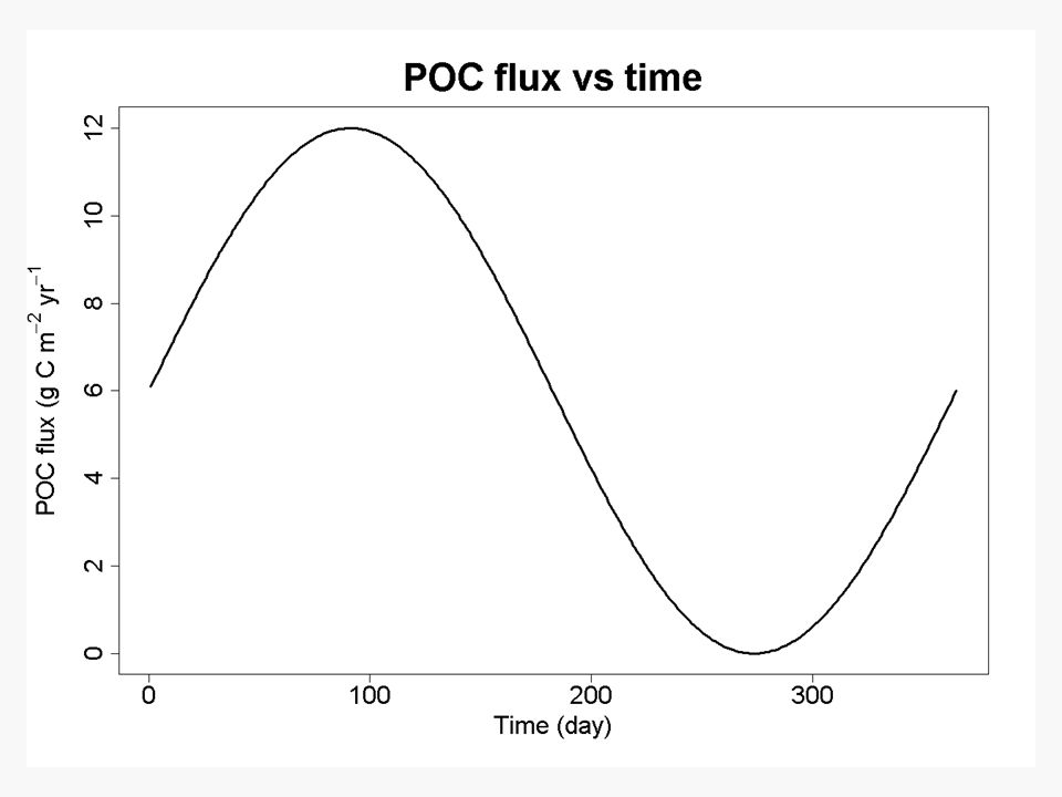


 Transport and Physical properties Sedimentation without diagenesis (reactions that alter solid composition.>")


 Deep-sea sediments: composition,>")
 Christoph Heinze University of Bergen, Geophysical Institute and Bjerknes Centre for Climate Research Prof. in.>")


