Financial Management I Review for FIN 338

Financial Management I Review for FIN 338
FIN 331 in a Nutshell Financial Management I Review for FIN 338

Time Value of Money Timelines Future Value Present Value
Present Value of Uneven Cash Flows

Time Lines: Timing of Cash Flows
1 2 3 I% CF0 CF1 CF2 CF3 Tick marks occur at the end of periods Time 0 = today Time 1 = the end of the first period or the beginning of the second period +CF = Cash INFLOW -CF = Cash OUTFLOW PMT = Constant CF

Basic Definitions Present Value (PV) Future Value (FV)
The current value of future cash flows discounted at the appropriate discount rate Value at t=0 on a time line Future Value (FV) The amount an investment is worth after one or more periods. “Later” money on a time line It’s important to point out that there are many different ways to refer to the interest rate that we use in time value of money calculations. Students often get confused with the terminology, especially since they tend to think of an “interest rate” only in terms of loans and savings accounts.

Future Value: General Formula
FV = PV(1 + I)N FV = future value PV = present value I = period interest rate, expressed as a decimal N = number of periods Future value interest factor = (1 + I)N Note: “yx” key on your calculator

Texas Instruments BA-II Plus
FV = future value PV = present value PMT = periodic payment I/Y = period interest rate N = number of periods One of these MUST be negative I am providing information on the Texas Instruments BA-II Plus – other calculators are similar. If you recommend or require a specific calculator other than this one, you may want to make the appropriate changes. Note: the more information students have to remember to enter the more likely they are to make a mistake. For this reason, I normally tell my students to set P/Y = 1 and leave it that way. Then I teach them to work on a period basis, which is consistent with using the formulas. If you want them to use the P/Y function, remind them that they will need to set it every time they work a new problem and that CLR TVM does not affect P/Y. If students are having difficulty getting the correct answer, make sure they have done the following: Set decimal places to floating point (2nd Format, Dec = 9 enter) or show 4 to 5 decimal places if using and HP Double check and make sure P/Y = 1 Make sure to clear the TVM registers after finishing a problem (or before starting a problem) It is important to point out that CLR TVM clears the FV, PV, N, I/Y and PMT registers. C/CE and CLR Work DO NOT affect the TVM keys The remaining slides will work the problems using the notation provided above for calculator keys. The formulas are presented in the notes section. N I/Y PV PMT FV

Excel Spreadsheet Functions
=FV(rate,nper,pmt,pv) =PV(rate,nper,pmt,fv) =RATE(nper,pmt,pv,fv) =NPER(rate,pmt,pv,fv) Use the formula icon (ƒx) when you can’t remember the exact formula Click on the tabs at the bottom of the worksheet to move between examples.

Future Values – Example
Suppose you invest $100 for 5 years at 10% How much would you have? Formula Solution: FV =PV(1+I)N =100(1.10)5 =100(1.6105) =161.05 It is important at this point to discuss the sign convention in the calculator. The calculator is programmed so that cash outflows are entered as negative and inflows are entered as positive. If you enter the PV as positive, the calculator assumes that you have received a loan that you will have to repay at some point. The negative sign on the future value indicates that you would have to repay in 5 years. Show the students that if they enter the 1000 as negative, the FV will compute as a positive number. Also, you may want to point out the change sign key on the calculator. There seem to be a few students each semester that have never had to use it before. Formula: FV = 1000(1.05)5 = 1000( ) =

Future Value – Example Suppose you invest $100 for 5 years at 10%. How much would you have? Calculator Solution 5 N 10 I/Y -100 PV 0 PMT CPT FV = It is important at this point to discuss the sign convention in the calculator. The calculator is programmed so that cash outflows are entered as negative and inflows are entered as positive. If you enter the PV as positive, the calculator assumes that you have received a loan that you will have to repay at some point. The negative sign on the future value indicates that you would have to repay in 5 years. Show the students that if they enter the 1000 as negative, the FV will compute as a positive number. Also, you may want to point out the change sign key on the calculator. There seem to be a few students each semester that have never had to use it before. Formula: FV = 1000(1.05)5 = 1000( ) =

Future Value: Important Relationship 1
For a given interest rate: The longer the time period, The higher the future value FV = PV(1 + I)N Remember the sign convention. Formulas: PV = 500 / (1.1)5 = 500( ) = PV = 500 / (1.1)10 = 500( ) = For a given I, as N increases, FV increases

Future Value Important Relationship 2
For a given time period: The higher the interest rate, The larger the future value FV = PV(1 + I)N Formulas: PV = 500 / (1.1)5 = 500( ) = PV = 500 / (1.15)5 = 500( ) = For a given N, as I increases, FV increases

Present Values The current value of future cash flows discounted at the appropriate discount rate Value at t=0 on a time line Answers the questions: How much do I have to invest today to have some amount in the future? What is the current value of an amount to be received in the future? Point out that the PV interest factor = 1 / (1 + r)t

PV = FV(1+I)-N FV = PV(1 + I)N Present Values
Rearrange to solve for PV PV = FV / (1+I)N PV = FV(1+I)-N “Discounting” = finding the present value of one or more future amounts Point out that the PV interest factor = 1 / (1 + r)t

Present Value: One Period Example
You need $10,000 for the down payment on a new car You can earn 7% annually. How much do you need to invest today? 1 N; 7 I/Y; 0 PMT; 10000 FV; CPT PV = PV = 10,000(1.07)-1 = 9,345.79 The students can read the example in the book. After carefully going over your budget, you have determined you can afford to pay $632 per month towards a new sports car. You call up your local bank and find out that the going rate is 1 percent per month for 48 months. How much can you borrow? Note that the difference between the answer here and the one in the book is due to the rounding of the Annuity PV factor in the book. =PV(0.07,1,0,10000)

Present Value: Important Relationship 1
For a given interest rate: The longer the time period, The lower the present value Remember the sign convention. Formulas: PV = 500 / (1.1)5 = 500( ) = PV = 500 / (1.1)10 = 500( ) = For a given I, as N increases, PV decreases

Present Value Important Relationship 2
For a given time period: The higher the interest rate, The smaller the present value Formulas: PV = 500 / (1.1)5 = 500( ) = PV = 500 / (1.15)5 = 500( ) = For a given N, as I increases, PV decreases

The Basic PV Equation - Refresher
PV = FV / (1 + I)N There are four parts to this equation PV, FV, I and N Know any three, solve for the fourth If you are using a financial calculator, be sure and remember the sign convention +CF = Cash INFLOW -CF = Cash OUTFLOW

Multiple Cash Flows Present Value
The Basic Formula The TI BA II+ Using the PV/FV keys Using the Cash Flow Worksheet Excel

Multiple Uneven Cash Flows Present Value
You are offered an investment that will pay $200 in year 1, $400 the next year, $600 the following year, and $800 at the end of the 4th year. You can earn 12% on similar investments. What is the most you should pay for this investment? FV = 100(1.08) (1.08)2 = =

What is the PV of this uneven cash flow stream?
200 1 400 2 600 3 12% 800 4 -1, = PV

Present Value of an Uneven Cash Flow Stream: Formula

Multiple Uneven Cash Flows – PV
Year 1 CF: 1 N; 12 I/Y; 200 FV; CPT PV = Year 2 CF: 2 N; 12 I/Y; 400 FV; CPT PV = Year 3 CF: 3 N; 12 I/Y; 600 FV; CPT PV = Year 4 CF: 4 N; 12 I/Y; 800 FV; CPT PV = Total PV = -$1,432.93

Multiple Uneven Cash Flows – Using the TI BAII’s Cash Flow Worksheet
Clear all: Press CF Then 2nd And CLR WORK (above CE/C) CF0 is displayed and is 0 Enter the Period 0 cash flow If it is an outflow, hit “+/-” to change the sign To enter the figure in the cash flow register, press ENTER

TI BAII+: Uneven CFs Press the down arrow () to move to the next cash flow register. Enter the cash flow amount, press ENTER and then down arrow to move to the cash flow counter (Fn). The default counter value is “1”. To accept the value of “1”, press the down arrow again. To change the counter, enter the correct count, press ENTER and then the down arrow.

TI BAII+: Uneven CFs Repeat for all cash flows, in order. To find NPV:
Press NPV: I appears on the screen Enter the interest rate, press ENTER and the down arrow to display NPV. Press compute “CPT”

TI BAII+: Uneven Cash Flows
CF0 = 0 CF1 = 200 CF2 = 400 CF3 = 600 CF4 = 800 CF C00 0 ENTER  C ENTER  F01 1 ENTER  C ENTER  F02 1 ENTER  C ENTER  F03 1 ENTER  C ENTER  F04 1 ENTER  NPV I 12 ENTER  NPV CPT

Excel – PV of multiple uneven CFs

CHAPTER 3 Financial Statements, Cash Flow, and Taxes
Key Financial Statements Balance sheet Income statements Statement of cash flows

The Annual Report Balance sheet Income statement
Snapshot of a firm’s financial position at a point in time Income statement Summarizes a firm’s revenues and expenses over a given period of time Statement of cash flows Reports the impact of a firm’s activities on cash flows over a given period of time

Sample Balance Sheet Assets = Liabilities + Owner’s Equity
Olympic’s balance sheet is pretty straightforward. Assets consist of cash and cash equivalents, short-term investments, accounts receivable and inventories under current assets plus net plant and equipment. Liabilities include accounts payable, notes payable, and accruals under current liabilities plus Olympic has long-term bonds outstanding. Shareholder (common) equity includes both common stock and retained earnings consistent with the basic balance sheet equation: Assets = Liabilities plus Equity As is fairly typical, we report Olympic’s balance sheet numbers for two consecutive years – 2007 and 2008.

Sample Income Statement
Olympic’s Income statements for 2007 and 2008 are on this slide. Consistent with our goal of keeping these statements simple and basic, Olympic’s income statement is uncomplicated. Beginning with top line net sales, we subtract operating costs to arrive at gross profit. Subtracting depreciation and other operating expenses yields operating income. Subtracting interest expense results in pretax income. Applying the corporate tax rate of 40%, we arrive at the bottom line, net income. Note that net income is divided between common dividends and addition to retained earnings. Net income=Dividends + Retained earnings

Allied Food Products

Allied 2005 Per-Share Ratios
Formula & Calculation Earnings per Share (EPS) Dividends per Share (DPS) Book Value per Share (BVPS) Cash flow per Share (CFPS) This slide recaps Olympic’s Per-Share Ratios for 2008. Olympic has 50 million shares outstanding. Note that Operating Cash Flow used in computing cash flow per share is equal to net income plus depreciation.

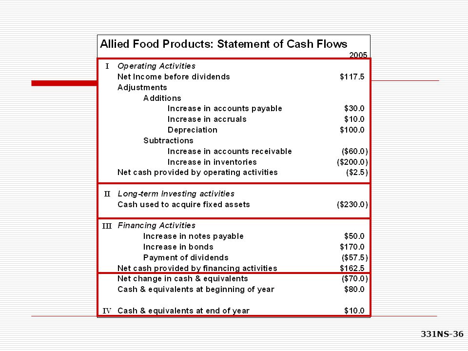
Statement of Cash Flows
Provides information about cash inflows and outflows during an accounting period Required since 1988 Developed from Balance Sheet and Income Statement data

Reconciles the change in Cash & Equivalents

Why is it important??? Reconciles the Income Statement and Balance Sheet to the flow of cash The Matching Principle requires estimates and accruals to prepare Financial statements Financial Analysis is concerned with Cash Flow

“A positive net income on the income statement is ultimately insignificant unless a company can translate its earnings into cash, and the only source in financial statement data for learning about the generation of cash from operations is the statement of cash flows”

Covered by new debt and cash
Deficits Covered by new debt and cash

Net Operating Working Capital

Operating Capital (also called Total Net Operating Capital)
= NOWC + Net fixed assets (2005) = $800 + $1,000 = $1,800 million (2004) = $650 + $ = $1,520 million Net Investment in Operating Capital = Op Cap (2005) – Op Cap (2004) = $1,800 - $1,520 = $280 million

Net Operating Profit after Taxes (NOPAT) & Operating Cash Flow
NOPAT = EBIT(1 - Tax rate) NOPAT05 = $283.8( ) = $170.3 m OCF05 = NOPAT + Deprec + Amort = $ $100 = $270.3

Free Cash Flow (FCF) for 2005
EBIT = $283.8 m T = 40% Depreciation = $100 m Capital Expenditures = FA + Deprec = $130+$100 = $230 NOWC = $800 - $650 = $150 m FCF = [$283.8(1-.4)+$100] –[$230-$150] = -$109.7 m

CHAPTER 4 Analysis of Financial Statements
Ratio Analysis Limitations of ratio analysis Qualitative factors

Five Major Categories of Ratios
Liquidity CR - Current Ratio QR - Quick Ratio or “Acid-Test” Asset management Inventory Turnover DSO – Days sales outstanding FAT - Fixed Assets Turnover TAT - Total Assets Turnover Debt management Debt Ratio TIE – Times interest earned EBITDA coverage (EC)

Five Major Categories of Ratios
Profitability PM - Profit margin on sales BEP – Basic earning power ROA – Return on total assets ROE – Return on common equity Market value P/E – Price-Earnings ratio P/CF – Price – cash flow ratio M/B – Market to book

Liquidity Ratios CR = Current Ratio QR = Quick Ratio or “Acid-Test”
= CA/CL QR = Quick Ratio or “Acid-Test” = (CA-INV)/CL

Asset Management Ratios
Inventory Turnover = Sales/Inventories DSO = Days sales outstanding = Receivables /(Annual sales/365) FAT = Fixed Assets Turnover = Sales/Net Fixed Assets TAT = Total Assets Turnover = Sales/Total Assets

Debt Management Ratios
Debt Ratio = Total Liabilities/Total Assets TIE = Times interest earned = EBIT/Interest EBITDA coverage = EC (EBITDA + lease pmts) (Interest + principal pmts + lease pmts)

Profitability Ratios = NI/Sales = EBIT/Total Assets = NI/Total Assets
PM = Profit margin on sales = NI/Sales BEP = Basic earning power = EBIT/Total Assets ROA = Return on total assets = NI/Total Assets ROE = Return on common equity = NI/Common Equity

Market Value Metrics Book value per share P/E = Price-Earnings ratio
= Price per share/Earnings per share P/CF = Price–cash flow ratio = Price per share/Cash flow per share M/B = Market to book = Market price per share Book value per share

The 5 Major Categories of Ratios and What Questions They Answer
Ratio Category Questions Answered Liquidity Can we make required payments? Asset Management Right amount of assets vs. sales? Debt Management Right mix of debt and equity? Profitability Do sales prices exceed unit costs Are sales high enough as reflected in PM, ROE, and ROA? Market Value Do investors like what they see as reflected in P/E and M/B ratios

Potential Problems and Limitations of Ratio Analysis
Comparison with industry averages is difficult if the firm operates many different divisions “Average” performance ≠ necessarily good Seasonal factors can distort ratios Window dressing techniques

Problems and Limitations (Continued)
Different accounting and operating practices can distort comparisons Sometimes difficult to tell if a ratio value is “good” or “bad” Different ratios give different signals Difficult to tell, on balance, whether a company is in a strong or weak financial condition

Qualitative Factors Revenues tied to a single customer?
Revenues tied to a single product? Reliance on a single supplier? Percentage of business generated overseas? Competitive situation? Legal and regulatory environment?

CHAPTER 16 Financial Planning and Forecasting
Forecasting sales Projecting the assets and internally generated funds Projecting outside funds needed Deciding how to raise funds

The AFN Formula If ratios are expected to remain constant:
AFN = (A*/S0)∆S - (L*/S0)∆S - M(S1)(RR) Required  Assets  Retained Earnings Spontaneously  Liabilities

Variables in the AFN Formula
A* = Assets tied directly to sales S0 = Last year’s sales S1 = Next year’s projected sales ∆S = Increase in sales; (S1-S0) L* = Liabilities that spontaneously increase with sales

Variables in the AFN Formula
A*/S0: assets required to support sales; “Capital Intensity Ratio” L*/S0: spontaneous liabilities ratio M: profit margin (Net income/sales) RR: retention ratio; percent of net income not paid as dividend

Key Factors in AFN ∆S = Sales Growth A*/S0 = Capital Intensity Ratio
L*/S0 = Spontaneous Liability Ratio M = Profit Margin RR = Retention Ratio

CHAPTER 6 Interest Rates

“Nominal” vs. “Real” rates
r = Any nominal rate r* = The “real” risk-free rate ≈ T-bill rate with no inflation Typically ranges from 1% to 4% per year rRF = Rate on Treasury securities Proxied by T-bill or T-bond rate

r = r* + IP + DRP + LP + MRP rRF = Here:
r = Required rate of return on a debt security r* = Real risk-free rate IP = Inflation premium DRP = Default risk premium LP = Liquidity premium MRP = Maturity risk premium rRF =

Premiums Added to r* for Different Types of Debt
Debt Instrument IP DRP MRP LP ST Treasury ST IP LT Treasury LT IP MRP ST Corporate ST IP DRP LP LT Corporate LT IP DRP MRP LP

CHAPTER 7 Bonds and Their Valuation
Bond valuation Measuring yield

Discount Rate = YTM The discount rate (YTM) is: For debt securities:
The opportunity cost of capital The rate that could be earned on alternative investments of equal risk Required return For debt securities: YTM = r* + IP + LP + MRP + DRP

Bond Value Bond Value = PV(coupons) + PV(par)
Bond Value = PV(annuity) + PV(lump sum) Remember: As interest rates increase present values decrease – as YTM ↑ → PV ↓ As interest rates increase, bond prices decrease and vice versa

The Bond-Pricing Equation
This formalizes the calculations we have been doing. PV(lump sum) PV(Annuity) C = Coupon payment; F = Face value

Texas Instruments BA-II Plus
FV = future value/face value/par value PV = present value=bond value/price I/Y = period interest rate = YTM N = number of periods to maturity PMT = coupon payment I am providing information on the Texas Instruments BA-II Plus – other calculators are similar. If you recommend or require a specific calculator other than this one, you may want to make the appropriate changes. Note: the more information students have to remember to enter the more likely they are to make a mistake. For this reason, I normally tell my students to set P/Y = 1 and leave it that way. Then I teach them to work on a period basis, which is consistent with using the formulas. If you want them to use the P/Y function, remind them that they will need to set it every time they work a new problem and that CLR TVM does not affect P/Y. If students are having difficulty getting the correct answer, make sure they have done the following: Set decimal places to floating point (2nd Format, Dec = 9 enter) or show 4 to 5 decimal places if using and HP Double check and make sure P/Y = 1 Make sure to clear the TVM registers after finishing a problem (or before starting a problem) It is important to point out that CLR TVM clears the FV, PV, N, I/Y and PMT registers. C/CE and CLR Work DO NOT affect the TVM keys The remaining slides will work the problems using the notation provided above for calculator keys. The formulas are presented in the notes section. N I/Y PV PMT FV

Spreadsheet Functions
FV(Rate,Nper,Pmt,PV,0/1) PV(Rate,Nper,Pmt,FV,0/1) RATE(Nper,Pmt,PV,FV,0/1) NPER(Rate,Pmt,PV,FV,0/1) PMT(Rate,Nper,PV,FV,0/1) Click on the tabs at the bottom of the worksheet to move between examples. Inside parens: (RATE,NPER,PMT,PV,FV,0/1) “0/1” Ordinary annuity = 0 (default) Annuity Due = 1 (must be entered)

Pricing Specific Bonds
TI BA II+ Bond Worksheet [2nd] BOND SDT CPN RDT RV ACT 2/Y YLD PRI Excel: PRICE(Settlement,Maturity,Rate,Yld,Redemption, Frequency,Basis) YIELD(Settlement,Maturity,Rate,Pr,Redemption, Frequency,Basis) Settlement and maturity need to be actual dates Redemption and Pr need to given as % of par value Please note that you have to have the analysis tool pack add-ins installed to access the PRICE and YIELD functions. If you do not have these installed on your computer, you can use the PV and the RATE functions to compute price and yield as well. Click on the TVM tab to find these calculations.

Yield to Maturity (YTM)
The market required rate of return for bonds of similar risk and maturity The discount rate used to value a bond Return earned if bond held to maturity Usually = coupon rate at issue Quoted as an APR The IRR of a bond

Must find the rd that solves this model:
What is the YTM on a 10-year, 9% annual coupon, $1,000 par value bond, selling for $887? Must find the rd that solves this model:

Using a financial calculator to solve for the YTM
Bond sells at a discount because YTM > coupon rate 10 - 887 90 1000 INPUTS N I/YR PV PMT FV OUTPUT 10.91

Solving for YTM YTM on a 10-year, 9% annual coupon, $1,000 par value bond selling for $887 Using the calculator: N = 10 PV = -887 PMT = 90 FV = 1000 CPT I/Y = 10.91 Coupon rate = 9% Annual coupons Par = $1,000 Maturity = 10 years Price = $887 Remember the sign convention on the calculator. The easy way to remember it with bonds is we pay the PV (-) so that we can receive the PMT (+) and the FV(+). Slide 7.8 discusses why this bond sells at less than par =RATE(10,90,-887,1000)

Find YTM, if the bond price is $1,134.20
Bond sells at a premium because YTM < coupon rate 10 90 1000 INPUTS N I/YR PV PMT FV OUTPUT 7.08

Solving for YTM YTM on a 10-year, 9% annual coupon, $1,000 par value bond selling for $1,134.20 Coupon rate = 9% Annual coupons Par = $1,000 Maturity = 10 years Price = $1,134.20 Using the calculator: N = 10 PV = PMT = 90 FV = 1000 CPT I/Y = 7.08 Remember the sign convention on the calculator. The easy way to remember it with bonds is we pay the PV (-) so that we can receive the PMT (+) and the FV(+). Slide 7.8 discusses why this bond sells at less than par =RATE(10,90, ,1000)

Semiannual bonds 2N rd / 2 OK cpn / 2 OK INPUTS N I/YR PV PMT FV
Multiply years by 2 : number of periods = 2N. Divide nominal rate by 2 : periodic rate (I/YR) = rd / 2. Divide annual coupon by 2 : PMT = ann cpn / 2. 2N rd / 2 OK cpn / 2 OK INPUTS N I/YR PV PMT FV OUTPUT

What is the value of a 10-year, 10% semiannual coupon bond, if rd = 13%?
Multiply years by 2 : N = 2 * 10 = 20 Divide nominal rate by 2 : I/YR = 13 / 2 = 6.5 Divide annual coupon by 2 : PMT = 100 / 2 = 50 20 6.5 50 1000 INPUTS N I/YR PV PMT FV OUTPUT

Valuing a Semiannual Bond
Coupon rate = 10% Annual coupons Par = $1,000 Maturity = 10 years YTM = 13% Using the calculator: N = 20 I/Y = 6.5 PMT = 50 FV = 1000 CPT PV = Using the formula: Remember the sign convention on the calculator. The easy way to remember it with bonds is we pay the PV (-) so that we can receive the PMT (+) and the FV(+). Slide 7.8 discusses why this bond sells at less than par =PV(0.065, 10, 50, 1000)

YTM with Semiannual Coupons
Suppose a bond with a 10% coupon rate and semiannual coupons, has a face value of $1000, 20 years to maturity and is selling for $ Is the YTM more or less than 10%? What is the semiannual coupon payment? How many periods are there?

YTM with Semiannual Coupons
Suppose a bond with a 10% coupon rate and semiannual coupons, has a face value of $1000, 20 years to maturity and is selling for $ N = 40 PV = PMT = 50 FV = 1000 CPT I/Y = 4% YTM = 4%*2 = 8%  Result = ½ YTM NOTE: Solving a semi-annual payer for YTM will result in a 6-month YTM answer Calculator solves what you enter.

CHAPTER 8 Risk and Rates of Return
Stand-alone Risk Portfolio Risk Risk & Return: CAPM / SML

The Expected Rate of Return
r “hat” = expected return ri = expected return in “ith” state of the economy Pi = Probability of “ith” state occurring

Calculating the Expected Return

The Standard Deviation of Returns
σ = √ Variance = √ σ2

Standard deviation for each investment

Standard Deviation of HT’s Returns

Risk versus Return: Do we know enough now?
Security Expected return, r Risk, σ T-bills 5.5% 0.0% HT 12.4% 20.0% Coll 1.0% 13.2% USR 9.8% 18.8% Market 10.5% 15.2% ^

Coefficient of Variation (CV)
CV = Standard deviation/expected return = Risk per unit of return =

Portfolio Expected Return
^ rp = weighted average wi = % of portfolio in stock i ri = return on stock i 18

Portfolio Expected Return
Assume a two-stock portfolio is created with $50,000 invested in both HT and Collections ^ rp = 0.5(12.4%) + 0.5(1.0%) = 6.7%

Portfolio Return “Portfolio” = (50% x HT) + (50% x Coll)
“Portfolio Return” = Prob x “Portfolio”

Portfolio Risk Portfolio Standard deviation is NOT a weighted average of the standard deviations of the component assets

Calculating portfolio standard deviation and CV

Portfolio Standard Deviation

Portfolio Risk & Return
 σp = 3.4% is much lower than the σ of either stock σp = 3.4% is lower than the weighted average of HT and Coll.’s σ (16.6%) The portfolio provides the average return of component stocks, but lower than the average risk Why? Negative correlation between stocks

Covariance of Returns Measures how much the returns on two risky assets move together

Covariance vs. Variance of Returns

Covariance Covariance (HT:Coll) =

Correlation Coefficient
Correlation Coefficient = ρ (rho) Scales covariance to [-1,+1] -1 = Perfectly negatively correlated 0 = Uncorrelated; not related +1 = Perfectly positively correlated

Two-Stock Portfolios If r = -1.0 If r = +1.0
Two stocks can be combined to form a riskless portfolio If r = +1.0 No risk reduction at all In general, stocks have r ≈ 0.35 Risk is lowered but not eliminated Investors typically hold many stocks 22

s of n-Stock Portfolio Subscripts denote stocks i and j
ri,j = Correlation between stocks i and j σi and σj =Standard deviations of stocks i and j σij = Covariance of stocks i and j

Portfolio Risk-n Risky Assets
i j for n=2 1 1 w1w111 = w1212 1 2 w1w212 2 1 w2w121 2 2 w2w222 = w2222 p2 = w1212 + w2222 + 2w1w2 12

Portfolio Risk-2 Risky Assets

Capital Asset Pricing Model (CAPM)
Links risk and required returns Security Market Line (SML): A stock’s required return equals the risk-free return (rRF) plus a risk premium (RPM x ) that reflects the stock’s risk after diversification Primary conclusion: The relevant riskiness of a stock is its contribution to the riskiness of a well-diversified portfolio.

The SML and Required Return
The Security Market Line (SML) is part of the Capital Asset Pricing Model (CAPM) rRF = Risk-free rate RPM = Market risk premium = rM – rRF 43

The Market Risk Premium (rM – rRF = RPM)
Additional return over the risk-free rate to compensate investors for assuming an average amount of risk Size depends on: Perceived risk of the stock market Investors’ degree of risk aversion Varies from year to year Estimates suggest a range between 4% and 8% per year

Required Rates of Return
Assume: rRF = 5.5% RPM = 5% rHT = 5.5% + (5.0%)(1.32) = 5.5% + 6.6% = 12.10% rM = 5.5% + (5.0%)(1.00) = 10.50% rUSR = 5.5% + (5.0%)(0.88) = % rT-bill = 5.5% + (5.0%)(0.00) = % rColl = 5.5% + (5.0%)(-0.87) = %

Expected vs Required Returns
“Required” by the market “Expected” by YOU Expected Required Return HT 12.40 12.10 Undervalued Market 10.50 Fairly valued USR 9.80 9.90 Overvalued T-bills 5.50 Coll 1.00 1.15

Illustrating the Security Market Line
SML: ri = 5.5% + (5.0%) i ri (%) SML . HT . . rM = 10.5 rRF = 5.5 . USR T-bills . Risk, i Coll.

Portfolio Beta Where: wi = weight (% dollars invested in asset i)
βi = Beta of asset i βp = Portfolio Beta 47

CHAPTER 9 Stocks and Their Valuation

Constant growth stock Dividends expected to grow forever at a constant rate, g: D1 = D0 (1+g)1 D2 = D0 (1+g)2 Dt = D0 (1+g)t Dividend growth formula converges to:

Constant Growth Model Needed data: D0 = Dividend just paid
D1 = Next expected dividend g = constant growth rate rs = required return on the stock

Expected Value at time t

Supernormal Growth What if g = 30% for 3 years before achieving long-run growth of 6%? Constant growth model no longer applicable But - growth constant after 3 years

Valuing common stock with nonconstant growth
1 2 3 4 D0 = ... 4.658 rs = 13% g = 30% g = 6% 2.301 2.647 3.045 46.114 = P0 = 0.06 $66.54 3 4.658 0.13 - $ P ^

Corporate Value Model = Free Cash Flow method
Value of the firm = present value of the firm’s expected future free cash flows Free cash flow =after-tax operating income less net capital investment FCF = NOPAT – Net capital investment

Applying the corporate value model
Market value of firm: (MVF) = PV(future FCFs) MV of common stock: = MVF – MV of debt Intrinsic stock value: = MVCS /# shares

Issues regarding the corporate value model
Often preferred to the dividend growth model Firms that don’t pay dividends Dividends hard to forecast Assumes at some point free cash flow growth rate will be constant Terminal value (TVN) = value of firm at the point that growth becomes constant

Firm’s Intrinsic Value
Long-run gFCF = 6% WACC = 10% 21.20 1 2 3 4 ... g = 6% r = 10% -4.545 8.264 15.026 21.20 530 = = TV3 0.10 0.06 -

MV of equity = MV of firm – MV of debt = $416.94 - $40
If the firm has $40 million in debt and has 10 million shares of stock, what is the firm’s intrinsic value per share? MV of equity = MV of firm – MV of debt = $ $40 = $ million Value per share= MV of equity / # of shares = $ / 10 = $37.69

Firm multiples method Often used by analysts to value stocks
P / E Price-earning P / CF Price-cash flow P / Sales Price-sales Method: Estimate appropriate ratio based on comparable firms Multiply estimate by expected metric to estimate stock price

CHAPTER 10 The Cost of Capital
Cost of equity WACC Adjusting for risk

WACC Weighted Average Cost of Capital
WACC = wdrd(1-T) + wprp + wcrs Where: wD = % of debt in capital structure wP= % of preferred stock in capital structure wC= % of common equity in capital structure rD = firm’s cost of debt rP= firm’s cost of preferred stock rC= firm’s cost of equity T = firm’s corporate tax rate Weights Component costs

Three ways to determine the cost of equity, rs:
1. DCF: rs = D1/P0 + g 2. CAPM: rs = rRF + (rM - rRF)βi = rRF + (RPM)βi 3. Own-Bond-Yield-Plus-Risk Premium: rs = rd + Bond RP

DCF Approach: Inputs Current stock price (P0) Current dividend (D0)
Growth rate (g)

Four Mistakes to Avoid Use Target weights Use market value of equity
Current (YTM) vs. historical (Coupon rate) cost of debt Mixing current and historical measures to estimate the market risk premium Book weights vs. Market Weights Use Target weights Use market value of equity Book value of debt = reasonable proxy for market value. Incorrect cost of capital components Only investor provided funding

A firm’s composite WACC reflects the risk of an average project
Should the company use the composite WACC as the hurdle rate for each of its projects? NO! A firm’s composite WACC reflects the risk of an average project WACC = “hurdle rate” for an average risk project Different divisions/projects may have different risks Division or project WACC should be adjusted to reflect appropriate risk

Divisional and Project Costs of Capital
Using the WACC as the discount rate is only appropriate for projects that are the same risk as the firm’s current operations If considering a project that is NOT of the same risk as the firm, then an appropriate discount rate for that project is needed Divisions also often require separate discount rates It is important to point out that the WACC is not very useful for companies that have several disparate divisions. www: Click on the web surfer icon to go to an index of business owned by General Electric. Ask the students if they think that projects proposed by “GE Infrastructure” should have the same discount rate as projects proposed by “GE Healthcare.” You can go through the list and illustrate why the divisional cost of capital is important for a company like GE. If GE’s WACC was used for every division, then the riskier divisions would get more investment capital and the less risky divisions would lose the opportunity to invest in positive NPV projects.

Using WACC for All Projects - Example
What would happen if we use the WACC for all projects regardless of risk? Assume the WACC = 15% Ask students which projects would be accepted if they used the WACC for the discount rate? Compare 15% to IRR and accept projects A and B. Now ask students which projects should be accepted if you use the required return based on the risk of the project? Accept B and C. So, what happened when we used the WACC? We accepted a risky project that we shouldn’t have and rejected a less risky project that we should have accepted. What will happen to the overall risk of the firm if the company does this on a consistent basis? Most students will see that the firm will become riskier.

Divisional Risk and the Cost of Capital
Rate of Return (%) Acceptance Region WACC WACC H Acceptance Region Rejection Region WACC F Rejection Region WACC L Risk Risk Risk L H

Subjective Approach Consider the project’s risk relative to the firm overall If project risk > firm risk  project discount rate > WACC If project risk < firm risk  project discount rate < WACC

Subjective Approach - Example
Risk Level Discount Rate Very Low Risk WACC – 8% % Low Risk WACC – 3% % Same Risk as Firm WACC % High Risk WACC + 5% % Very High Risk WACC + 10% %

CHAPTER 11 The Basics of Capital Budgeting
Should we build this plant?

Steps to capital budgeting
Estimate CFs (inflows & outflows) Assess riskiness of CFs Determine appropriate cost of capital Find NPV and/or IRR Accept if NPV>0 and/or IRR>WACC

Independent versus Mutually Exclusive Projects
The cash flows of one are unaffected by the acceptance of the other Mutually Exclusive: The acceptance of one project precludes acceptance of the other

NPV: Sum of the PVs of all cash flows.
∑ n t = 0 CFt (1 + r)t . NOTE: t=0 Cost often is CF0 and is negative NPV = ∑ n t = 1 CFt (1 + r)t - CF0

TI BAII+: Uneven Cash Flows
CF0 = -100 CF1 = 10 CF2 = 60 CF3 = 80 CF C /- ENTER  C ENTER  F01 1 ENTER  C ENTER  F02 1 ENTER  C ENTER  F03 1 ENTER NPV I 10 ENTER  NPV CPT $18.78

Internal Rate of Return (IRR)
IRR = the discount rate that forces PV of inflows equal to cost, and the NPV = 0: Solving for IRR with a financial calculator: Enter CFs in CFLO register Press IRR:

∑ ∑ NPV vs IRR NPV: Enter r, solve for NPV CFt = NPV (1 + r)t
IRR: Enter NPV = 0, solve for IRR = 0 ∑ n t = 0 CFt (1 + IRR)t

Modified Internal Rate of Return (MIRR)
MIRR = discount rate which causes the PV of a project’s terminal value (TV) to equal the PV of costs TV = inflows compounded at WACC MIRR assumes cash inflows reinvested at WACC

Normal vs. Non-normal Cash Flows
Normal Cash Flow Project: Cost (negative CF) followed by a series of positive cash inflows One change of signs Non-normal Cash Flow Project: Two or more changes of signs Most common: Cost (negative CF), then string of positive CFs, then cost to close project For example, nuclear power plant or strip mine

Multiple IRRs Descartes Rule of Signs 1 real root per sign change
Polynomial of degree n→n roots 1 real root per sign change Rest = imaginary (i2 = -1)

The Pavillion Project: Non-normal CFs and MIRR
1 2 -800,000 5,000,000 -5,000,000 PV 10% = -4,932,231.40 TV 10% = 5,500,000.00 MIRR = 5.6%

MIRR versus IRR MIRR correctly assumes reinvestment at opportunity cost = WACC MIRR avoids the multiple IRR problem Managers like rate of return comparisons, and MIRR is better for this than IRR

When to use the MIRR instead of the IRR? Accept Project P?
When there are nonnormal CFs and more than one IRR, use MIRR. PV of 10% = -$4, TV of 10% = $5,500. MIRR = 5.6%. Do not accept Project P. NPV = -$ < 0. MIRR = 5.6% < WACC = 10%.

Excel Functions

Cash Flow Estimation and Risk Analysis
CHAPTER 12 Cash Flow Estimation and Risk Analysis 150

Relevant Cash Flows: Incremental Cash Flow for a Project
Project’s incremental cash flow is: Corporate cash flow with the project Minus Corporate cash flow without the project

Relevant Cash Flows Changes in Net Working Capital…… Y
Interest/Dividends …………..………….. N “Sunk” Costs ………………………………….. N Opportunity Costs ………………………….Y Externalities/Cannibalism …………….. Y Tax Effects ………………………..………….. Y

Tax Effect on Salvage Net Salvage Cash Flow = SP - (SP-BV)(T) Where:
SP = Selling Price BV = Book Value T = Corporate tax rate 153

Including inflation when estimating cash flows
Nominal r > real r The cost of capital, r, includes a premium for inflation Nominal CF > real CF Nominal cash flows incorporate inflation If you discount real CF with the higher nominal r, then your NPV estimate is too low

Real vs. Nominal Cash flows
INFLATION Real vs. Nominal Cash flows Real Nominal 155

Real vs. Nominal Cash flows
INFLATION Real vs. Nominal Cash flows 2 Ways to adjust Adjust WACC Cash Flows = Real Adjust WACC to remove inflation Adjust Cash Flows for Inflation Use Nominal WACC 156

Sensitivity Analysis Shows how changes in an input variable affect NPV or IRR Each variable is fixed except one Change one variable to see the effect on NPV or IRR Answers “what if” questions

Sensitivity Analysis

Sensitivity Graph Variable Cost Unit Sales Fixed Cost

Sensitivity Ratio If SR>0  Direct relationship
14-162 Sensitivity Ratio %NPV = (New NPV - Base NPV)/Base NPV %VAR = (New VAR - Base VAR)/Base VAR If SR>0  Direct relationship If SR<0  Inverse relationship 162

Sensitivity Ratio -30% $ -62 $54 $266 SR 13.74 -5.72 -41.22
14-163 Sensitivity Ratio Change from Resulting NPV (000s) Base Level Unit Sales FC VC -30% $ -62 $54 $266 %NPV (-62-20)/ (54-20)/20 (266-20)/ % % % %VAR % % % SR 163

Sensitivity Graph Variable Cost -41.22 Unit Sales 13.74 Fixed Cost
-5.72

Results of Sensitivity Analysis
Steeper sensitivity lines = greater risk Small changes → large declines in NPV The Variable Cost line is steeper than unit sales or fixed cost so, for this project, the firm should focus on the accuracy of variable cost forecasts.

Sensitivity Analysis: Weaknesses
Does not reflect diversification Says nothing about the likelihood of change in a variable i.e. a steep sales line is not a problem if sales won’t fall Ignores relationships among variables

Sensitivity Analysis: Strengths
Provides indication of stand-alone risk Identifies dangerous variables Gives some breakeven information

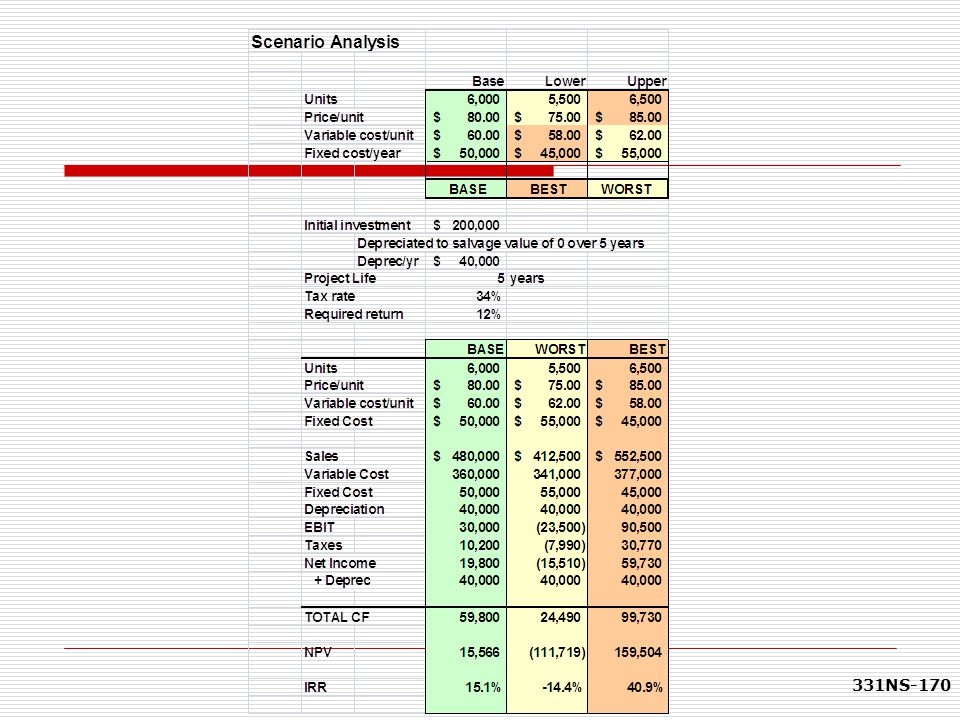
Scenario Analysis Examines several possible situations, usually:
Worst case Base case or most likely case, and Best case Provides a range of possible outcomes

Scenario Example

Problems with Scenario Analysis
Only considers a few possible out-comes Assumes that inputs are perfectly correlated All “bad” values occur together and all “good” values occur together Focuses on stand-alone risk

Monte Carlo Simulation Analysis
Computerized version of scenario analysis using continuous probability distributions Computer selects values for each variable based on given probability distributions

Monte Carlo Simulation Analysis
Calculates NPV and IRR Process is repeated many times (1,000 or more) End result: Probability distribution of NPV and IRR based on sample of simulated values Generally shown graphically

Histogram of Results

Advantages of Simulation Analysis
Reflects the probability distributions of each input Shows range of NPVs, the expected NPV, σNPV, and CVNPV Gives an intuitive graph of the risk situation

Disadvantages of Simulation Analysis
Difficult to specify probability distributions and correlations If inputs are bad, output will be bad: “Garbage in, garbage out”

Disadvantages of Sensitivity, Scenario and Simulation Analysis
Sensitivity, scenario, and simulation analyses do not provide a decision rule Do not indicate whether a project’s expected return is sufficient to compensate for its risk Sensitivity, scenario, and simulation analyses all ignore diversification Measure only stand-alone risk, which may not be the most relevant risk in capital budgeting

Real Options When managers can influence the size and risk of a project’s cash flows by taking different actions during the project’s life in response to changing market conditions Alert managers always look for real options in projects Smarter managers try to create real options

Types of Real Options Investment timing options Growth options
Expansion of existing product line New products New geographic markets Abandonment options Contraction Temporary suspension Flexibility options

Financial Management I Review for FIN 338
FIN 331 in a Nutshell Financial Management I Review for FIN 338

Financial Management I Review for FIN 338

Similar presentations

Presentation on theme: "Financial Management I Review for FIN 338"— Presentation transcript:

Similar presentations

About project

Feedback

Log in

Auth with social network:

Financial Management I Review for FIN 338

Similar presentations

Presentation on theme: "Financial Management I Review for FIN 338"— Presentation transcript:

Similar presentations

About project

Feedback