1. Chapter 9A Process Capability and Statistical Quality Control
Process Variation
Process Capability
Process Control Procedures
Variable data
Attribute data
Acceptance Sampling
Operating Characteristic Curve

2. Basic Causes of Variation
Assignable causes are factors that can be clearly identified and possibly managed.
Common causes are inherent to the production process. In order to reduce variation due to common causes, the process must be changed.
Key: Determining which is which!

3. Types of Control Charts
Attribute (Go or no-go information)
Defectives refers to the acceptability of product across a range of characteristics.
p-chart application
Variable (Continuous)
Usually measured by the mean and the standard deviation.
X-bar and R chart applications

4. Types of Statistical Quality Control
Process
Process
Acceptance
Acceptance
Control
Control
Sampling
Sampling
Variables
Variables
Attributes
Attributes
Variables
Variables
Attributes
Attributes
Charts
Charts
Charts
Charts

5. Excellent review in exhibit TN8.5.
Statistical Process Control (SPC) Charts
UCL
LCL
Samples over time
Normal Behavior
Look for trends!
UCL
LCL
Samples over time
Possible problem, investigate
Excellent review in exhibit TN8.5.
UCL
LCL
Samples over time
Possible problem, investigate

6. Control Limits
We establish the Upper Control Limits (UCL) and the Lower Control Limits (LCL) with plus or minus 3 standard deviations. Based on this we can expect 99.7% of our sample observations to fall within these limits. x
LCL
UCL
99.7%

7. Example of Constructing a p-Chart: Required Data
Sample
Sample size
Number of defectives

8. Statistical Process Control Formulas: Attribute Measurements (p-Chart)
Given:
Compute control limits:

9. Example of Constructing a p-chart: Step 1
1. Calculate the sample proportions, p (these are what can be plotted on the p-chart) for each sample.

10. Example of Constructing a p-chart: Steps 2&3
2. Calculate the average of the sample proportions.
3. Calculate the standard deviation of the sample proportion

11. Example of Constructing a p-chart: Step 4
4. Calculate the control limits.
UCL =
LCL = (0)

12. Example of Constructing a p-Chart: Step 5
5. Plot the individual sample proportions, the average
of the proportions, and the control limits

13. R Chart Type of variables control chart Shows sample ranges over time
Interval or ratio scaled numerical data
Shows sample ranges over time
Difference between smallest & largest values in inspection sample
Monitors variability in process
Example: Weigh samples of coffee & compute ranges of samples; Plot

14. R Chart Control Limits From Table (function of sample size)
Sample Range in sample i
# Samples

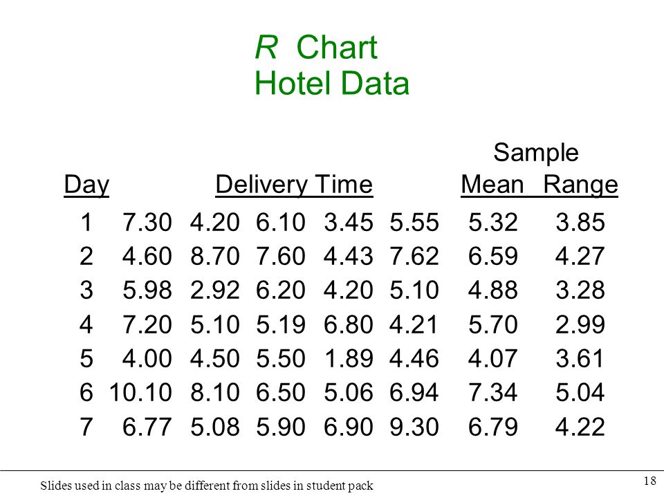
15. R Chart Example
You’re manager of a 500-room hotel. You want to analyze the time it takes to deliver luggage to the room. For 7 days, you collect data on 5 deliveries per day. Is the process in control?

16. R Chart Hotel Data Sample Day Delivery Time Mean Range
Sample Mean =

17. R Chart Hotel Data Sample Day Delivery Time Mean Range
Largest
Smallest
Sample Range =

18. R Chart Hotel Data Sample Day Delivery Time Mean Range

19. R Chart Control Limits Solution
From Table (n = 5)

20. R Chart Control Chart Solution
UCL
R-bar

21. X Chart Type of variables control chart Shows sample means over time
Interval or ratio scaled numerical data
Shows sample means over time
Monitors process average
Example: Weigh samples of coffee & compute means of samples; Plot

22. X Chart Control Limits
From Table
Mean of sample i
Range of sample i
# Samples

23. X Chart Example
You’re manager of a 500-room hotel. You want to analyze the time it takes to deliver luggage to the room. For 7 days, you collect data on 5 deliveries per day. Is the process in control?

24. X Chart Hotel Data Sample Day Delivery Time Mean Range

25. X Chart Control Limits Solution*
From Table
(n = 5)

26. X Chart Control Chart Solution*
UCL
X-bar
LCL

27. X AND R CHART EXAMPLE IN-CLASS EXERCISE
The following collection of data represents samples of the amount of force applied in a gluing process:
Determine if the process is in control
by calculating the appropriate upper and lower
control limits of the X-bar and R charts.

28. X AND R CHART EXAMPLE IN-CLASS EXERCISE

29. Example of x-bar and R charts: Step 1
Example of x-bar and R charts: Step 1. Calculate sample means, sample ranges, mean of means, and mean of ranges.

30. Example of x-bar and R charts: Step 2
Example of x-bar and R charts: Step 2. Determine Control Limit Formulas and Necessary Tabled Values

31. Example of x-bar and R charts: Steps 3&4
Example of x-bar and R charts: Steps 3&4. Calculate x-bar Chart and Plot Values

32. Example of x-bar and R charts: Steps 5&6: Calculate R-chart and Plot Values

33. SOLUTION: Example of x-bar and R charts:
1. Is the process in Control?
2. If not, what could be the cause for the process being out of control?

34. Process Capability
Process limits - actual capabilities of process based on historical data
Tolerance limits - what process design calls for - desired performance of process

35. Process Capability How do the limits relate to one another?
You want: tolerance range > process range
1. Make bigger
2. Make smaller
Two methods of accomplishing this:
Implies having greater control over process
Þ Good!
Bad idea

36. Process Capability Measurement
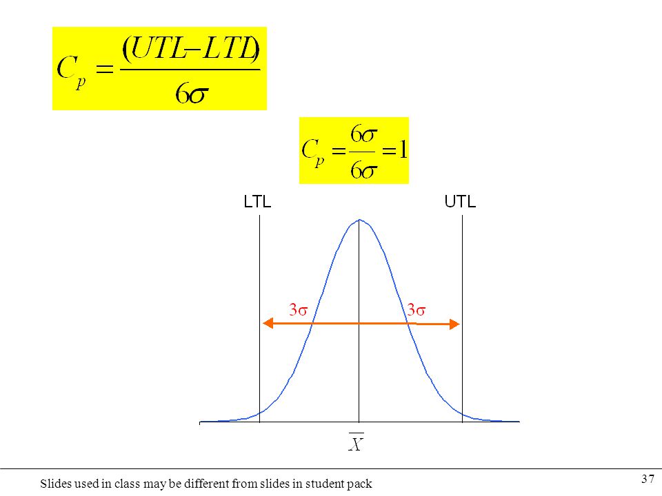
Cp index = Tolerance range / Process range
What value(s) would you like for Cp?
Þ Larger Cp indicates a more reliable and predictable process (less variability)
The Cp index is based on the assumption that the process mean is centered at the midpoint of the tolerance range

38. LTL
UTL

39. While the Cp index provides useful information on process variability, it does not give information on the process average relative to the tolerance limits. Note:
LTL
UTL

40. Cpk Index = process mean (Unknown but can be estimated
Refers to the LTL
Refers to the UTL
= process mean (Unknown but can be estimated
with the grand mean)
s = standard deviation (Unknown but can be
estimated with the average range)
Together, these process capability Indices show how well parts being produced conform to design specifications.

41. Since Cp and Cpk are different we can conclude that the process is not centered, however the Cp index tells us that the process variability is very low
LTL
UTL

42. An example of the use of process capability indices
The design specifications for a machined slot is 0.5± .003 inches. Samples have been taken and the process mean is estimated to be The process standard deviation is estimated to be .001.
What can you say about the capability of this process to produce this dimension?

43. Process capability Machined slot (inches) 0.497 inches 0.503 inches
LTL
0.503 inches
UTL
 = 0.001
inches
Process mean
0.501 inches

44. Sampling Distributions (The Central Limit Theorem)
Regardless of the underlying distribution, if the sample is large enough (>30), the distribution of sample means will be normally distributed around the population mean with a standard deviation of :

45. Computing Process Capability Indexes Using Control Chart Data
Recall the following info from our in class exercise:
Since A2 is calculated on the assumption of three sigma limits:

46. From the Central Limit Theorem:
So,
Therefore,

47. Suppose the Design Specs for the Gluing Process were 10. 7 
Suppose the Design Specs for the Gluing Process were 10.7  .2, Calculate the Cp and Cpk Indexes:
Answer:

48. Note, multiplying each component of the Cpk calculation by 3 yields a Z value. You can use this to predict the % of items outside the tolerance limits:
From Appendix E we would expect:
= .044 or 4.4%
non-conforming product from this process
.792 * 3 = 2.38
.597 * 3 = 1.79
.008 or .8% of the curve
.036 or 3.6% of the curve

49. Capability Index – In Class Exercise
You are a manufacturer of equipment. A drive shaft is purchased from a supplier close by. The blueprint for the shaft specs indicate a tolerance of 5.5 inches ± .003 inches. Your supplier is reporting a mean of inches. And a standard deviation of inches.
What is the Cpk index for the supplier’s process?

51. Your engineering department is sent to the supplier’s site to help improve the capability on the shaft machining process. The result is that the process is now centered and the CP index is now On a percentage basis, what is the improvement on the percentage of shafts which will be unusable (outside the tolerance limits)?

52. To answer this question we must determine the percentage of defective shafts before and after the intervention from our engineering department

53. Before: From Table From Table .004 .089 Total % outside
(3x.88) =2.67s
3x.444 = 1.33s
Total % outside
Tolerance = = .093 or 9.3% -4

54. After
Since the process is centered then Cpk = Cp; Cp = UTL-LTL / 6s, so the tolerance limits are .75 x 6s = 4.5s apart each 2.25s from the mean
From Table
.012
2.25s
2.25s
So % outside of
Tolerance =
.012(2) = .024
Or 2.4% -4

55. So the percentage decrease in defective parts is 1 – (2.4/9.3) = 74%

57. Basic Forms of Statistical Sampling for Quality Control
Sampling to accept or reject the immediate lot of product at hand (Acceptance Sampling).
Sampling to determine if the process is within acceptable limits (Statistical Process Control)

58. Acceptance Sampling Purposes Advantages Determine quality level
Ensure quality is within predetermined level
Advantages
Economy
Less handling damage
Fewer inspectors
Upgrading of the inspection job
Applicability to destructive testing
Entire lot rejection (motivation for improvement)

59. Acceptance Sampling Disadvantages
Risks of accepting “bad” lots and rejecting “good” lots
Added planning and documentation
Sample provides less information than 100-percent inspection
No information is obtained on the process. Just sorting “good” parts from “bad” parts

60. Risk Acceptable Quality Level (AQL) a (Producer’s risk)
Max. acceptable percentage of defectives defined by producer.
a (Producer’s risk)
The probability of rejecting a good lot.
Lot Tolerance Percent Defective (LTPD)
Percentage of defectives that defines consumer’s rejection point.
 (Consumer’s risk)
The probability of accepting a bad lot.