1. Managerial Statistics
Why are we all here?
In a classroom, near the beginning of an executive M.B.A. program in management, getting ready to start a course on …

2. The job of a manager is to make …
decisions.
What’s so hard about that?

3. Fundamental Fact of Life
causal relationships
the things we really care about
the things we directly control
are typically
NOT
So, why don’t we just give up?
What makes life worth living?
FAITH!

4. This Course
… is focused on a single statistical tool for studying relationships:
Regression Analysis
That said, we won’t use this tool until we reach the second section of the course.
First, we need to be comfortable with the two “languages” of statistics
The language of estimation (“trust”)
The language of hypothesis testing (“evidence”)

5. Our Four Sessions Together
The ideas underlying statistics, and the two languages of statistics
The “science” of regression analysis (how to use the tool)
The “art” of regression analysis (regression modeling – how to use the tool wisely and well)
More modeling

6. First Part of Class An overview of statistics
What is statistics?
Why is it done?
How is it done?
What is the fundamental idea behind all of it?
The language of estimation
Who cares?
Two technical issues, one of which can’t be avoided

7. What is “Statistics”?
Statistics is focused on making inferences about a group of individuals (the population of interest) using only data collected from a subgroup (the sample).
Why might we do this?
Perhaps …
the population is large, and looking at all individuals would be too costly or too time-consuming
taking individual measurements is destructive
some members of the population aren’t available for direct observation

8. Managers aren’t Paid to be Historians
Their concern is how their decisions will play out in the future.
Still, if the near-term future can be expected to be similar to the recent past, then the past can be viewed as a sample from a larger population consisting of both the recent past and the soon-to-come future.
The sample gives us insight into the population as a whole, and therefore into whatever the future holds in store.
Indeed, even if you stand in the middle of turbulent times, data from past similarly turbulent times may help you find the best path forward.

9. How is Statistics Done?
Any statistical study consists of three specifications:
How will the data be collected?
How much data will be collected in this way?
What will be computed from the data?
Running example: Estimating the average age across a population, in preparation for a sales pitch.

10. 1. How Will the Data be Collected?
Primary Goals: No bias High precision Low cost
Simple random sampling with replacement
Typically implemented via systematic sampling
Simple random sampling without replacement
Typically done if a population list is available
Covered in marketing research
Stratified sampling
Done if the population consists of subgroups with substantial within-group homogeneity
Cluster sampling
Done if the population consists of (typically geographic) subgroups with substantial within-group heterogeneity
Specialized approaches

11. 2. How is the Sample Size Chosen?
In order to yield the desired (target) precision (to be made clearer in a while)
simple random sampling with replacement
sample size of 5

12. 3. What Will be Done with the Data?
Some possible estimates of the population mean from the five observations:
median (third largest)
average of extremes ( [largest + smallest] / 2)
sample mean ( x = (x1+x2+x3+x4+x5)/5)
smallest (probably not a very good idea)

13. We’ve Finally Chosen an Estimation Procedure!
simple random sampling with replacement
sample size of 5
our estimate of the population mean will be the sample mean, x = (x1+x2+x3+x4+x5)/5
This will certainly give us an estimate.
But how much can we trust that estimate???

14. The Fundamental Idea underlying All of Statistics
At the moment I decide how I’m going to make an estimate, if I look into the future, the (not yet determined) end result of my chosen estimation procedure looks like a random variable. Using the tools of probability, I can analyze this random variable to see how precise my ultimate (after the procedure is carried out) estimate is likely to be.

15. Some Notation
population size, N mean,  standard deviation, , where 2=∑(xi-)2 / N
sample size, n sample mean, x sample standard deviation, s, where s2=∑(xi- x )2 / (n-1)

16. For Our Estimation Procedure, with X Representing the End Result
E[ X ] = 
our procedure is right, on average
StDev( X ) = /n
if this is small, our procedure typically gives an estimate close to 
X is approximately normally distributed
(from the Central Limit Theorem)

17. Pulling This All Together, Here’s the “Language” of Estimation
“I conducted a study to estimate {something} about {some population}. My estimate is {some value}. The way I went about making this estimate, I had {a large chance} of ending up with an estimate within {some small amount} of the truth.” For example, “I conducted a study to estimate the mean amount spent on furniture over the past year by current subscribers to our magazine. My estimate is $530. The way I went about making this estimate, I had a 95% chance of ending up with an estimate within $36 of the truth.”

18. Pictorially

19. For Simple Random Sampling with Replacement
“I conducted a study to estimate , the mean value of something that varies from one individual to the next across the given population. “My estimate is x . The way I went about making this estimate, I had a 95% chance of ending up with an estimate within 1.96·/n of the truth. “(And the other 5% of the time, I’d typically be off by only slightly more than this.)”

20. There’s Only One Problem …
We don’t know  ! So we cheat a bit, and use s (an estimate of  based on the sample data) instead. And so … Our estimate of  is x , and the margin of error (at the 95%-confidence level) is 1.96·s/n .

21. And That’s It!
We can afford to standardize our language of "trust" around the notion of 95% confidence, because translations to other levels of confidence are simple. The following statements are totally synonymous:
I'm 90%-confident that my estimate is wrong by no more than $   (~1.64)·s/√n
I'm 95%-confident that my estimate is wrong by no more than $   (~1.96)·s/√n    
I'm 99%-confident that my estimate is wrong by no more than $   (~2.58)·s/√n 

22. Next
Why should a manager want to know the margin of error in an estimate?
Some necessary technical details
Polling (estimating the proportion of the population with some qualitative property)
The language of hypothesis testing (evaluating evidence: to what extent does data support or contradict a statement?)

23. The Language of Estimation (for Simple Random Sampling with Replacement)
the standard error of the mean (one standard-deviation’s-worth of exposure to error when estimating the population mean)
the margin of error (implied, unless otherwise explicitly stated: at the 95%-confidence level) when the sample mean is used as an estimate of the population mean
a 95%-confidence interval for the population mean μ

24. To whom, and where, is the $36 margin of error of relevance?
Advertising Sales
A magazine publishing house wishes to estimate (for purposes of advertising sales) the average annual expenditure on furniture among its subscribers.
A sample of 100 subscribers is chosen at random from the 100,000-person subscription list, and each sampled subscriber is questioned about their furniture purchases over the last year. The sample mean response is $530, with a sample standard deviation of $180.
To whom, and where, is the $36 margin of error of relevance?

25. Put Yourself in the Shoes of the Marketing Manager at a Furniture Company
Part of your job is to track the performance of current ad placements. Each month …
You apportion sales across all the placements.
You divide sales by placement costs.
You rank the placements by “bang per buck.”
The lowest ranked placement is at the top of your replacement list, and its ratio determines the hurdle a new opportunity must clear to replace it.

26. Keep Yourself in the Shoes of the Marketing Manager at the Furniture Company
Another part of your job is to learn the relationship between properties of specific ad placements, and the performance of those placements.
You do this using regression analysis, with the characteristics of, and return on, previous placements as your sample data.
Given the characteristics of a new opportunity (e.g., number of subscribers to a magazine, and how much the average subscriber spends on furniture in a year), you can predict the likely return on your advertising dollar if you take advantage of this opportunity.

27. One Day, the Advertising Sales Representative for a Magazine Drops By
S/he wants you to buy space in this magazine. You ask (among other things), “What’s the average amount your subscribers spend on furniture per year?” S/he says, “ $530 ± $36 ” You put $530 (and other relevant information) into your regression model … and it predicts a return greater than your current hurdle rate! Do you jump onboard?

28. What If the $530 is an Over-Estimate or an Under-Estimate?
The predicted bang-per-buck could actually be worse than your hurdle rate!
There are many ways to do a risk analysis, and you’ll discuss them throughout the program. They all require that you know something about the uncertainty in numbers you’re using.
At the very least, you can put $494 and $566 into your prediction model, and see what you would predict in those cases.
[More generally, (margin-of-error/1.96) is one standard-deviation’s-worth of “noise” in the estimate. This can be used in more sophisticated analyses.]

29. Sometimes It’s Right to Say “Maybe”
If the prediction looks good at both extremes, you can be relatively confident that this is a good opportunity. If it looks meaningfully bad at either extreme, you delay your decision: “Gee! This sounds interesting, but your numbers are a bit too fuzzy for me to make a decision. Please go back and collect some more data. If the estimate stands up, and the margin of error can be brought down, I might be able to say “Yes.””

30. Practical Issues
If it looks good, either now or on a second visit, be sure to get details on the estimation study in writing as part of your deal. (Then you can sue for fraud if you learn the rep was lying.)
The risk analysis I’ve described is quite simplistic. You can (and will learn to) do better. But you’ll need the margin of error for any approach.

31. General Discussion
How would our answer ($530 ± $36) change, if there were 400,000 subscribers (instead of 100,000)?
It wouldn’t change at all! “N” doesn’t appear in our formulas.
The precision of our estimate depends on the sample size, but NOT on the size of the population being studied.
This is WONDERFUL!!!

32. (Continued) What if there had been only 4,000 subscribers?
Still no change.
What if there had been only 100 subscribers?
But wait!
Ahhh!! … Everything we’ve said so far, and the formulas we’ve derived, are for an estimation procedure involving simple random sampling with replacement.

33. Technical Detail #1
If we’d used simple random sampling without replacement:
E[ X wo] =  , the procedure is still right on average
StDev( X wo) = (/n)· : this is somewhat different!
X wo is still approximately normally distributed
(from the Central Limit Theorem)

34. For Simple Random Sampling without Replacement
But for typical managerial settings, this extra factor is just a hair less than 1. For example, if N = 100,000 and n = 100, the factor is
So in managerial settings the factor is usually ignored, and we’ll use
for both types of simple random sampling.

35. Technical Detail #2 twice! In coming up with , we cheated …
We invoked the Central Limit Theorem to get the 1.96, even though the CLT only says, “The bigger the bunch of things being aggregated, the closer the aggregate will come to having a normal distribution.”
As long as the sample size is a couple of dozen or more, OR even smaller when drawn from an approximately normal population distribution, this cheat turns out to be relatively innocuous.
We used s instead of .
This cheat is a bit more severe when the sample size is small. So we cover for it by raising the 1.96 factor a bit.
twice!

36. Very Technical Detail #2
By how much do we lift the 1.96 multiplier? To a number that comes from the t-distribution with n-1 “degrees of freedom.” This adjusts for using estimates of variability (such as s) instead of the actual variability (such as ), and for deriving these estimates from the same data already used to estimate other things (such as x for ).

37. Correcting for Using s Instead of 
t-distribution
degrees of freedom
95% central probability 1
12.706 11
2.201 21
2.080 2
4.303 12
2.179 22
2.074 3
3.182 13
2.160 23
2.069 4
2.776 14
2.145 24
2.064 5
2.571 15
2.131 25
2.060 6
2.447 16
2.120 30
2.042 7
2.365 17
2.110 40
2.021 8
2.306 18
2.101 60
2.000 9
2.262 19
2.093
120
1.980 10
2.228 20
2.086 ∞
1.960
Note that, as the sample size grows, the correct “approximately 2” multiplier becomes closer and closer to 1.96.

38. Pictorially

39. And How Do We Do This?
Fortunately, any decent statistical software these days will count degrees of freedom, look in the appropriate t-distribution tables, and give us the slightly-larger-than-1.96 number we should use. In general, just think
(one standard deviation’s worth of uncertainty in the way the estimate was made)
(your estimate) ± (~2) ·
as in
where the (~2) is determined by the computer

40. Imagine 100 teams, each trying to estimate the population mean (of a population which happens to actually have a true mean, unknown to the teams, of 75) using a sample size of 100.
Some will overestimate, and others will underestimate. But considering the margin of error in each estimate at the 95%-confidence level, we would expect only 5 of the 95 to be wrong by more than that margin of error. (Here, just by chance, only 4 were unlucky enough to miss by more than the margin of error.)

41. Here, with the same sample data, each makes the same estimate as before. But the margin of error at the 90%-confidence level is smaller.
Here, we’d expect about 10 to be off by that margin of error or more: Required to specify a smaller margin of error based on the same data, they must express less confidence that their actual error is below that smaller threshold.

42. Here, with the same sample data, each makes the same estimate as before. But the margin of error at the 99%-confidence level is larger.
Here, we’d expect about 1 to be off by that margin of error or more: Allowed to express a larger margin of error based on the same data, they can express more confidence that their actual error is below that larger threshold.

43. With a larger sample size (500), the margins of error at every level of confidence are smaller than before.

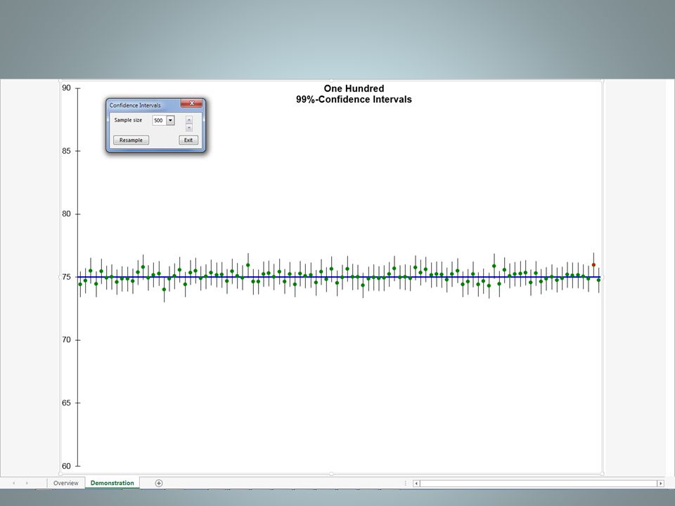
46. A Last Bit of Language ( the standard error of the
As we move forward, we’ll be making a variety of estimates and predictions. In each case, we’ll use the following terminology:
the standard error of the estimate or prediction =
one standard-deviation’s-worth of potential error
in our estimate or prediction due to random
“noise” in the estimation or prediction process
We’ll be running into the standard error of the mean, proportion, prediction, estimated mean, and coefficient at various times. The bottom line will always be that a 95%-confidence interval for our estimate or prediction is
( the standard error of the
estimate or prediction )
(your estimate or prediction) ± (~2) ·

47. Polling
If the individuals in the population differ in some qualitative way, we often wish to estimate the proportion / fraction / percentage of the population with some given property. For example: We track the sex of purchasers of our product, and find that, across 400 recent purchasers, 240 were female. What do we estimate to be the proportion of all purchasers who are female, and how much do we trust our estimate?

48. First, the Estimate
Let Obviously, this will be our estimate for the population proportion. But how much can this estimate be trusted?

49. And Now, the Trick
Imagine that each woman is represented by a “1”, and each man by a “0”. Then the proportion (of the sample or population) which is female is just the mean of these numeric values, and so estimating a proportion is just a special case of what we’ve already done!

50. The Result Estimating a mean: Estimating a proportion: The example:
[When all of the numeric values are either 0 or 1, s takes the special form shown above.]
The example:

51. Multiple-Choice Questions
If the Republican Party’s candidate were to be chosen today, which one would you most prefer?
Romney, Cain, Bachman, Perry, Gingrich, Santorum, Paul, Huntsman, none
The results are reported as if 9 separate “yes/no” questions had been asked.
If the Republican Party’s candidate were to be chosen today, which of these would have your approval?
The same reporting method is used.

52. Choice of Sample Size
Set a “target” margin of error for your estimate, based on your judgment as to how small will be small enough for those who will be using the estimate to make decisions.
There’s no magic formula here, even though this is a very important choice: Too large, and your study is useless; too small, and you’re wasting money.

53. Estimating a Proportion: Polling
Pick the target margin of error.
Why do news organizations always use 3% or 4% during the election season?
Because that’s the largest they can get away with.
So, for example, n=400 (resp., 625, or 1112) assures a margin of error of no more than 5% (resp., 4%, or 3%).

54. Estimating a Mean: Choice of Sample Size
Set the target margin of error.
Solve
From whence comes s?
From historical data (previous studies) or from a pilot study (small initial survey).
target = $25.
s  $180.
Set n = 207.

55. The “Square-Root” Effect : Choice of Sample Size after an Initial Study
Given the results of a study, to cut the margin of error in half requires roughly 4 times the original sample size.
And generally, the sample size required to achieve a desired margin of error =

56. How to Read Presidential-Race Polls
When reading political polls, remember that the margin of error in an estimate of the “gap” between the two leading candidates is roughly twice as large as the poll's reported margin of error.
The margin of error in the estimated “change in the gap” from one poll to the next is nearly three times as large as the poll's reported margin of error.

57. Summary
Whenever you give an estimate or prediction to someone, or accept an estimate or prediction from someone, in order to facilitate risk analysis be sure the estimate is accompanied by its margin of error: A95%-confidence interval is
If you’re estimating a mean using simple random sampling:
If you’re estimating a proportion using simple random sampling:
(one standard-deviation’s-worth of uncertainty inherent in the way the estimate was made)
(your estimate) ± (~2) ·

58. Hypothesis Testing
A statement has been made. We must decide whether to believe it (or not). Our belief decision must ultimately stand on three legs:
What does our general background knowledge and experience tell us (for example, what is the reputation of the speaker)?
What is the cost of being wrong (believing a false statement, or disbelieving a true statement)?
What does the relevant data tell us?

59. Making the “Belief” Decision
What does our general background knowledge and experience tell us (for example, what is the reputation of the speaker)? – The answer is typically already in the manager’s head.
What is the cost of being wrong (believing a false statement, or disbelieving a true statement)? – Again, the answer is typically already in the manager’s head.
What does the relevant data tell us? – The answer is typically not originally in the manager’s head. The goal of hypothesis testing is to put it there, in the simplest possible terms.
Then, the job of the manager is to pull these three answers together, and make the “belief” decision. The statistical analysis contributes to this decision, but doesn’t make it.

60. Our Goal is Simple:
To put into the manager’s head a single phrase which summarizes all that the data says with respect to the original statement.
“The data, all by itself, makes me ________ suspicious, because
the data, all by itself, contradicts the statement ________ strongly.”
{not at all, a little bit, moderately, quite, very, overwhelmingly}
We wish to choose the phrase which best fills the blanks.

61. What We Won’t Do What We Will Do
Compute Pr(statement is true | we see this data).
(This depends on our prior beliefs, instead of just on the data. It requires that we pull those beliefs out of the manager’s head.)
Compute Pr(we see this data | statement is true).
This depends just on the data. Since we don’t expect to see improbable things on a regular basis, a small value makes us very suspicious.
What We Will Do

62. This is Analogous to the British System of Criminal Justice
The statement on trial – the so-called “null hypothesis” – is that “the accused is innocent.”
The prosecution presents evidence.
The jury asks itself: “How likely is it that this evidence would have turned up, just by chance, if the accused really is innocent?”
If this probability is close to 0, then the evidence strongly contradicts the initial presumption of innocence … and the jury finds the accused “Guilty!”

63. Example: Processing a Loan Application
You’re the commercial loan officer at a bank, in the process of reviewing a loan application recently filed by a local firm. Examining the firm’s list of assets, you notice that the largest single item is $3 million in accounts receivable. You’ve heard enough scare stories, about loan applicants “manufacturing” receivables out of thin air, that it seems appropriate to check whether these receivables actually exist. You send a junior associate, Mary, out to meet with the firm’s credit manager.
Whatever report Mary brings back, your final decision of whether to believe that the claimed receivables exist will be influenced by the firm’s general reputation, and by any personal knowledge you may have concerning the credit manager. As well, the consequences of being wrong – possibly approving an overly-risky loan if you decide to believe the receivables are there and they’re not, or alienating a commercial client by disbelieving the claim and requiring an outside credit audit of the firm before continuing to process the application, when indeed the receivables are as claimed – will play a role in your eventual decision.

64. Processing a Loan Application
Later in the day, Mary returns from her meeting. She reports that the credit manager told her there were 10,000 customers holding credit accounts with the firm. He justified the claimed value of receivables by telling her that the average amount due to be paid per account was at least $300.
With his permission, she confirmed (by physical measurement) the existence of about 10,000 customer folders. (You decide to accept this part of the credit manager’s claim.) She selected a random sample of 64 accounts at random, and contacted the account-holders. They all acknowledged soon-to-be-paid debts to the firm. The sample mean amount due was $280, with a sample standard deviation of $120.
What do we make of this data? It contradicts the claim to some extent, but how strongly? It could be that the claim is true, and Mary simply came up with an underestimate due to the randomness of her sampling (her “exposure to sampling error”).

65. Compute, then Interpret
What do we make of Mary’s data? We answer this question in two steps.  First, we compute Pr(we see this data | statement is true). More precisely:
This number is called the significance level of the data, with respect to the statement under investigation (i.e., with respect to the null hypothesis). (Some authors/software call this significance level the “p-value” of the data.)
Then, we interpret the number:  A small value forces us to say, “Either the statement is true, and we’ve been very unlucky (i.e., we’ve drawn a very misrepresentative sample), or the statement is false.  We don’t typically expect to be very unlucky, so the data, all by itself, makes us quite suspicious.”
Pr (
conducting a study such as we just did, we’d see data at least as contradictory to the statement as the data we are, in fact, seeing |
the statement is true, in a way that fits the observed data as well as possible )

66. Null Hypothesis: “≥$300”
Mary’s sample mean is $280. Giving the original statement every possible chance of being found “innocent,” we’ll assume that Mary did her study in a world where the true mean is actually $300.
Let be the estimate Mary might have gotten, had she done her study in this assumed world.

67. the t-distribution with 63 degrees of freedom
The significance level of Mary’s data, with respect to the null hypothesis: “ ≥ $300”, is
The probability that Mary’s study would have yielded a sample mean of $280 or less, given that her study was actually done in a world where the true mean is $300.
 = $300
s/n = $120/64 = $15
the t-distribution with 63 degrees of freedom
9.36%

68. The “Hypothesis Testing Tool”
The spreadsheet “Hypothesis_Testing_Tool.xls,” in the “Session 1” folder, does the required calculations automatically.

69. And now, how do we interpret “9.36%”?
Coin_Tossing.htm
numeric significance level of the data  
interpretation: the data, all by itself, makes us  
the data supports the alternative hypothesis
above 20%
not at all suspicious
not at all
between 10% and 20%
a little bit suspicious
a little bit
between 5% and 10%
moderately suspicious
moderately
between 2% and 5%
very suspicious
strongly
between 1% and 2%
extremely suspicious
very strongly
below 1%
overwhelmingly suspicious
incredibly strongly

70. Processing a Loan Application
So the data, all by itself, makes us “a bit suspicious.” What do we do?
It depends.
If the credit manager is a trusted lifelong friend …
If the credit manager is already under suspicion …
What if Mary’s sample mean were $260?
With a significance level of 0.49%, the data, all by itself, makes us “overwhelmingly suspicious” …

71. The One-Sided Complication
A jury never finds the accused “innocent.”
For example, if the prosecution presents no evidence at all, the jury simply finds the accused “not proven to be guilty.”
Just so, we never conclude that data supports the null hypothesis.
However, if data contradicts the null hypothesis, we can conclude that it supports the alternative.

72. So, If We Wish to Say that Data Supports a Claim …
We take the opposite of the claim as our null hypothesis, and see if the data contradicts that opposite. If so, then we can say that the data supports the original claim.
Examples:
A clinical test of a new drug will take as the null hypothesis that patients who take the drug are equally or less healthy than those who don’t.
An evaluation of a new marketing campaign will take as the null hypothesis that the campaign is not effective.

73. And That’s It!
With the languages of estimation and hypothesis testing in place, it’s time to learn REGRESSION ANALYSIS!