Download presentation
Presentation is loading. Please wait.

1
Income Inequality: Measures, Estimates and Policy Illustrations

2
Focus of the Discussion:
Framework: Kuznets’: explain inequality in terms of inter-sectoral disparities & intra-sectoral inequalities Final outcome measures: Income generation: Sectoral perspective at the macro as well as disaggregate regional (district) level Income distribution Proxy: consumption distribution - macro (state), regional and district levels by rural/urban sectors
 level. Income distribution. Proxy: consumption distribution - macro (state), regional and district levels by rural/urban sectors.")
3
Inequality Measures & Welfare Judgments
Inequality measures have implicit normative judgments about inequality and the relative importance to be assigned to different parts of the income distribution. Some measures are clearly unattractive: Range: measures the distance between the poorest and richest; is y unaffected by changes in the distribution of income between these two extremes.

4
Simpler (statistical) measures
(normalised) Range Relative mean deviation (Shows percentage of total income that would need to be transferred to make all incomes are the same.) Coefficient of variation = standard deviation/mean 75-25 gap, gap
 Range. Relative mean deviation. (Shows percentage of total income that would need to be transferred to make all incomes are the same.) Coefficient of variation = standard deviation/mean gap, gap.")
5
Inequality measurement: Some attractive axioms
Pigou-Dalton Condition (principle of transfers): a transfer from a poorer person to a richer person, ceteris paribus, must cause an increase in inequality. Range does not satisfy this property. Scale-neutrality: Inequality should remain invariant with respect to scalar transformation of incomes. Variance does not satisfy this is property. Anonymity: Inequality measure should remain invariant with respect to any permutation.
: a transfer from a poorer person to a richer person, ceteris paribus, must cause an increase in inequality. Range does not satisfy this property. Scale-neutrality: Inequality should remain invariant with respect to scalar transformation of incomes. Variance does not satisfy this is property. Anonymity: Inequality measure should remain invariant with respect to any permutation.")
6
Gini coeficient Gini coeficient: The proportion of the total area under the Lorenz curve. Discrete version: Interpretation: Gini of “X” means that the expected difference in income btw. 2 randomly selected persons is 60% of overall mean income. Restrictive: -- The welfare impact of a transfer of income only depends on “relative rankings” – e.g., a transfer from the richest to the billionth richest household counts as much as one from the billionth poorest to the poorest.

7
The Atkinson class of inequality measures
Atkinson (1970) introduces the notion of ‘equally distributed equivalent’ income, YEDE. YEDE represents the level of income per head which, if equally shared, would generate the same level of social welfare as the observed distribution. A measure of inequality is given by: IA = 1- (YEDE/μ)
 introduces the notion of ‘equally distributed equivalent’ income, YEDE. YEDE represents the level of income per head which, if equally shared, would generate the same level of social welfare as the observed distribution. A measure of inequality is given by: IA = 1- (YEDE/μ)")
8
The Atkinson class of inequality measures
A low value of YEDE relative to μ implies that if incomes were equally distributed the same level of social welfare could be achieved with much lower average income.; IA would be large. Everything hinges on the degree of inequality aversion in the social welfare function. With no aversion, there is no welfare gain from edistribution so YEDE is equal to μ and IA = 0.

9
The Atkinson class of inequality measures
Atkinson proposes the following form for his inequality measure:

10
Atkinson’s measure This is just an iso-elastic social welfare function defined over income (not utility) with parameter e, normalised by average income
 with parameter e, normalised by average income.")
11
The Atkinson class of inequality measures
A key role here is played by the distributional parameter ε. In calculating IA you need to explicitly specify a value for ε. When ε=0 there is no social concern about inequality and so IA = 0 (even if the distribution is “objectively” unequal). When ε=∞ there is infinite weight to the poorer members of the population (“Rawls”)
. When ε=∞ there is infinite weight to the poorer members of the population ( Rawls )")
12
Inequality measurement and normative judgements
Coefficient of variation: Attaches equal weights to all income levels No less arbitrary than other judgments. Standard deviation of logarithms: Is more sensitive to transfers in the lower income brackets. Bottom line: The degree of inequality cannot in general be measured without introducing social judgments.

13
Theil’s Entropy Index Formally, an index I(Y) is Theil decomposable if: Where Yi is a the vector of incomes of the Hi members of subgroup i, there are N subgroups, and mieHi is an Hi long vector of the average income (mi) in subgroup i. The terms wi terms are subgroup weights. Theil’s Entropy Index:
 in subgroup i. The terms wi terms are subgroup weights. Theil’s Entropy Index:")
14
Recommendations No inequality measure is purely ‘statistical’: each embodies judgements about inequality at different points on the income scale. To explore the robustness of conclusions: Option 1: measure inequality using a variety of inequality measures (not just Gini). Option 2: employ the Atkinson measure with multiple values of ε. Option 3: look directly at Lorenz Curves, apply Stochastic Dominance results.
. Option 2: employ the Atkinson measure with multiple values of ε. Option 3: look directly at Lorenz Curves, apply Stochastic Dominance results.")
15
The Lorenz Curve To compare inequality in two distributions:
Plot the % share of total income received by the poorest nth percentile population in the population, in turn for each n and each consumption distribution. The greater the area between the Lorenz curve and the hypotenuse the greater is inequality. Second Order Stochastic Dominance (Atkinson 1970): If Lorenz curves for two distributions do not intersect, then they can be ranked irrespective of which measure of inequality is the focus of attention. If the Lorenz curves intersect, different summary measures of inequality can be found that will rank the distributions differently.
: If Lorenz curves for two distributions do not intersect, then they can be ranked irrespective of which measure of inequality is the focus of attention. If the Lorenz curves intersect, different summary measures of inequality can be found that will rank the distributions differently.")
16
Inequality Measures Shortcomings of GDP can be addressed in part by considering inequality Common measures of inequality Distribution of Y by Decile or Quintile

17
Income Distribution by Decile Group: Mexico, 1992

18
Inequality Measures Shortcomings of GDP can be addressed in part by considering inequality Common measures of inequality Distribution of Y by Decile or Quintile Gini Coefficient most commonly used summary statistic for inequality

19
Gini Coefficient 100 Lorenz Curve 100 Cumulative Income Share
100 Cumulative Population Share (poorest to riches)
")
20
Gini Coefficient 100 Lorenz Curve 1 Lorenz Curve 2 100
Cumulative Income Share 100 Cumulative Population Share

21
Gini Coefficient Gini = A / A + B A B 100 Lorenz Curve 100
Cumulative Income Share Gini = A / A + B A B 100 Cumulative Population Share

22
Gini Coefficient Gini varies from 0 - 1
Higher Ginis represent higher inequality The Gini is only a summary statistic, it doesn’t tell us what is happening over the whole distribution

23
Inequality Measures Shortcomings of GDP can be addressed in part by considering inequality Common measures of inequality Distribution of Y by Decile or Quintile Gini Coefficient most commonly used summary statistic for inequality Functional distribution of income

24
Inequality: Policy Instrument
Illustrate How Policy Strategies are made Little Realizing that the Very Framework used does not permit such an Approach Illustrate How Wrong Inferences are drawn on Empirical Estimates of Inequality, which finally form the basis for theoretically implausible Strategies for Poverty Reduction

25
DOES SPECIFICATION MATTER?
CHOICE OF STRATEGIES ESIMATES OF MAGNITUDES EVALUATION OF POLICY CONSEQUENCES ILLUSTRATED WITH REFERENCE TO THE INDIAN EXPERIENCE ON POLICIES FOR POVERTY REDUCTION, ESTIMATES & EVALUATION

26
CHOICE OF DEVT STRATEGIES
GROWTH WITH REDISTRIBUTION FORMULATED AND PURSUED INDEPENDENTLY BASED ON THE PREMISES OF SEPARABILITY AND INDEPENDENCE EXAMPLES: FIFTH & SIXTH FIVE YEAR PLANS

27
INDIAN SIXTH PLAN STRATEGY
RURAL INDIA: BASE YEAR (BY): BY POVERTY % TERMINAL YEAR (TY): REDUE TY POVERTY TO % BY GROTH (15.44 %) FURTHER DOWN TO 30 % BY REDISTRIBUTION (BY REDUCING INEQUALITY FROM TO 0.222)
: BY POVERTY % TERMINAL YEAR (TY): REDUE TY POVERTY TO % BY GROTH (15.44 %) FURTHER DOWN TO 30 % BY REDISTRIBUTION (BY REDUCING INEQUALITY FROM TO 0.222)")
28
INDIAN SIXTH PLAN STRATEGY
URBAN INDIA: BASE YEAR (BY): BY POVERTY % TERMINAL YEAR (TY): REDUE TY POVERTY TO % BY GROTH (11.32 %) FURTHER DOWN TO 30 % BY REDISTRIBUTION (BY REDUCING INEQUALITY FROM TO 0.305)
: BY POVERTY % TERMINAL YEAR (TY): REDUE TY POVERTY TO % BY GROTH (11.32 %) FURTHER DOWN TO 30 % BY REDISTRIBUTION (BY REDUCING INEQUALITY FROM TO 0.305)")
29
Growth with Redistribution
Base Year Terminal Year: HCR (%) Growth (%) Inequality change (%) Rural India 50.7 15.4 40.5 -27.4 30 Urban India 40.3 11.3 33.7 -8.8
 Growth (%) Inequality change (%) Rural India Urban India")
30
HOW VALID ARE THE PREMISES?
THE STRATEGIES ARE NEITHER SEPARABLE NOR INDEPENDENT GROWTH WILL REDUCE POVERTY AT AN INCREASING RATE IF HCR < 50% AT A DECREASING RATE IF HCR > 50% MAXIMUM IF HCR = 50%

31
RELATION BETWEEN GROWTH & POVERTY
1/2 ln x*

32
AN INCREASE IN INEQUALITY WILL:
INCREASE POVERTY AT A DECREASING RATE IF HCR < 50% DECREASE POVERTY AT AN INCREASING RATE IF HCR > 50% NEUTRAL WHEN HCR = 50%

33
RELATION BETWEEN INEQUALITY & POVERTY
1/2 1 P* For ln x* < For ln x* >

34
GROWTH vs. REDISTRIBUTION
GROWTH ALWAYS REDUCES POVERTY PACE OF REDUCION VARIES BETWEEN LEVELS OF DEVT. REDISTRIBUTION REDUCES POVERTY ONLY WHEN THE SIZE OF THE CAKE ITSELF IS LARGE ENOUGH & POVERTY < 50%

35
What are the Bases for Indian Devt. Strategy?
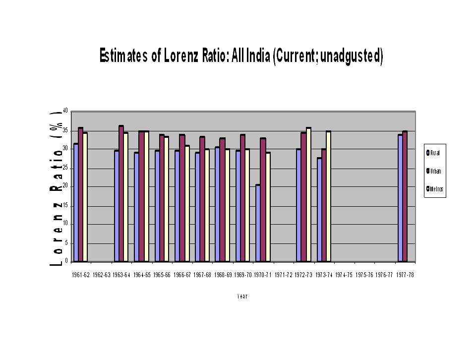
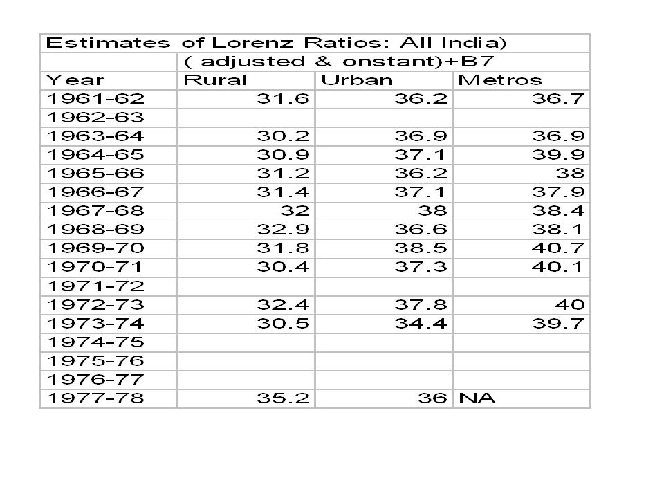
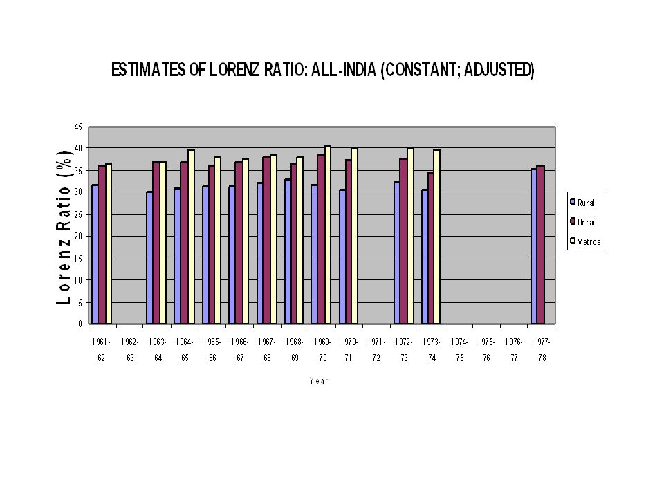
GROWTH & REDUCTION IN INEQUALITY INEQUALITY, AS MEASURED BY LORENZ RATIO, DECLINED AT THE RATE OF 0.38 % PER ANNUM IN RURAL INDIA DURING AND INEQUALITY DECLINED AT THE RATE OF 0.59% PER ANNUM IN URBAN INDIA DURING THE SAME PERIOD

38
How Valid are the Estimates?
ESTIMATES ARE BASED ON THE NATIONAL SAMPLE SURVEY (NSS) DATA ON CONSUMER EXPENDITURE NSS DATA ARE AVAILABLE ONLY IN GROUP FORM, THAT IS, IN THE FORM OF SIZE DISTRIBUTION OF POPULATION ACROSS MONTHLY EXPENDITURE CLASSES LORENZ RATIOS ARE ESTIMATED USING THE TRAPEZOIDAL RULE
 DATA ON CONSUMER EXPENDITURE. NSS DATA ARE AVAILABLE ONLY IN GROUP FORM, THAT IS, IN THE FORM OF SIZE DISTRIBUTION OF POPULATION ACROSS MONTHLY EXPENDITURE CLASSES. LORENZ RATIOS ARE ESTIMATED USING THE TRAPEZOIDAL RULE.")
39
Lorenz Ratio

40
Limitations: UNDERESTIMATES THE CONVEXITY OF THE LORENZ CURVE;
IN OTHER WORDS, IGNORES INEQUALITY WITHIN EACH EXPENDITURE CLAS HENCE, UNDERESTIMATES THE EXTENT OF INEQUALITY THE EXTENT OF UNDERESTIMATION INCREASES WITH THE WIDTH OF THE CLAS INTERVAL

41
NSS Monthly Per Capita Expenditure (PCE) Classes
Expenditure Class Population (%) PCE(Rs) < 8 8 – 11 11 – 13 13 – 15 15 – 18 18 – 21 21 – 24 24 – 28 28 –34 43 – 55 55 –75 > &5
 PCE(Rs) < 8. 8 – – – – – – – – – –75. > &5.")
42
Consumption Distribution: Metros 91961/62 & 1970/71)
Expenditure Class 1961/62 1970/71 < 8 (-) 8 – 11 0.89 (0.18) 11 – 13 1.21 (0.31) 0.24 (0.04) 13 – 15 1.44 (0.43) (-) 15 – 18 5.79 (1.99) 1.09 (0.27) 18 – 21 6.24 (2.53) 2.41 (0.70) 21 – 24 8.16 (3.86) 1.77 (0.60) 24 – 28 8.79 (4.82) 6.55 (2.50) 28 –34 12.55 (8.02) 7.38 (3.43) 13.15 (10.36) 17.55 (9.88) 43 – 55 14.31 (14.47) 13.61 (9.52) 55 –75 12.30 (16.36) 18.27 (17.91) > &5 15.17 (36.67) 31.13 (55.15)
 8 – (0.18) 11 – (0.31) 0.24 (0.04) 13 – (0.43) - (-) 15 – (1.99) 1.09 (0.27) 18 – (2.53) 2.41 (0.70) 21 – (3.86) 1.77 (0.60) 24 – (4.82) 6.55 (2.50) 28 – (8.02) 7.38 (3.43) (10.36) (9.88) 43 – (14.47) (9.52) 55 – (16.36) (17.91) > & (36.67) (55.15)")
43
Lorenz Curve: Indian Metros 1961/62 (current unadjusted)
")
44
Lorenz Curve: Indian Metros 1970/71 (Current unadjusted)
")
Similar presentations


 Jawaharlal Nehru University (JNU) New Delhi India>")


: - Growth is good for the poor irrespective of the.>")


