Warning: Very Mathematical!

Warning: Very Mathematical!
Factor Analysis Warning: Very Mathematical!

Motivating Example: McMaster’s Family Assessment Device
Consider the McMaster’s Family Assessment Device. It consists of 60 questions all on 4-point ordinal scale. On some items a high score indicates good family functioning, while others are indicative of lower functioning. Obviously many of the questions have some things in common and collectively measure different aspects of family functioning.

Motivating Example: McMaster’s Family Assessment Device (Q1-Q12)
We can see the positive family traits measured by the even-numbered items and the negative family traits measured by the odd-numbered items are positively correlated amongst themselves and negatively correlated with each other as expected.

Motivating Example: McMaster’s Family Assessment Device
But what does a subjects responses across all 12-items truly measure? We could simply add the items together, after reversing the scaling on the items that relate to the negative aspects of family functioning and family member interactions. After doing this a low total score would indicate a “good” family and a high total score would indicate a “bad” family. But perhaps there are different aspects of family functioning that the survey is measuring.

Factor Analysis Factor analysis is used to illuminate the underlying dimensionality of a set of measures. Some of these questions may cluster together to potentially measure things such things as communication, collaboration, closeness, or commitment. This is the idea behind factor analysis.

Factor Analysis Data reduction tool
Removes redundancy or duplication from a set of correlated variables. Represents correlated variables with a smaller set of “derived” variables. These derived variables may measure some underlying features of the respondents. Factors are formed that are relatively independent of one another. Two types of “variables”: latent variables: factors observed variables (items on the survey)

Applications of Factor Analysis
1. Identification of Underlying Factors: clusters variables into homogeneous sets creates new variables (i.e. factors) allows us to gain insight to categories 2. Screening of Variables: identifies groupings to allow us to select one variable to represent many useful in regression and other subsequent analyses

Applications of Factor Analysis
3. Summary: flexibility in being able to extract few or many factors 4. Sampling of variables: helps select small group of variables of representative yet uncorrelated variables from larger set to solve practical problem 5. Clustering of objects: “inverse” factor analysis, we will see an example of this when examining a car model perception survey.

“Perhaps the most widely used (and misused) multivariate
statistic is factor analysis. Few statisticians are neutral about this technique. Proponents feel that factor analysis is the greatest invention since the double bed, while its detractors feel it is a useless procedure that can be used to support nearly any desired interpretation of the data. The truth, as is usually the case,lies somewhere in between. Used properly, factor analysis can yield much useful information; when applied blindly, without regard for its limitations, it is about as useful and informative as Tarot cards. In particular, factor analysis can be used to explore the data for patterns, confirm our hypotheses, or reduce the many variables to a more manageable number.” -- Norman Streiner, PDQ Statistics

One Factor Model Classical Test Theory Idea:
Ideal: X1 = F + e1 var(ej) = var(ek) , j ≠ k X2 = F + e2 … Xp = F + ep Reality: X1 = λ1F + e1 var(ej) ≠ var(ek) , j ≠ k X2 = λ2F + e2 Xp = λpF + ep (unequal “sensitivity” to change in factor)

Key Concepts F is latent (i.e. unobserved, underlying) variable called a factor. X’s are the observed variables. ej is measurement error for Xj. λj is the “loading” on factor F for Xj.

Optional Assumptions We will make these to simplify our discussions
X’s are standardized prior to beginning a factor analysis, i.e. converted to z-scores. F is also standardized, that is the standard deviation of F is 1 and the mean is 0.

Some math associated with the ONE factor model
λj2 is also called the “communality” of Xj in the one factor case (Standard notation for communality: hj2) For standardized Xj , Corr(F, Xj) = λj For standardized variables, the percentage of variability in Xj explained by F is λj2. (like an R2 in regression) If Xj is N(0,1) or at least standardized, then λj is equivalent to: the slope in a regression of Xj on F the correlation between F and Xj Interpretation of λj: standardized regression coefficient (regression) path coefficient (path analysis) factor loading (factor analysis)

Some more math associated with the ONE factor model
Corr(Xj , Xk )= λjλk Note that the correlation between Xj and Xk is completely determined by the common factor F. Factor loadings (λj) are equivalent to correlation between factors and variables when only a SINGLE common factor is involved.

Example: McMaster’s FAD
For the 12-items of McMaster’s FAD used in this survey we can see that the one factor solution essentially reverses the scales of the items measuring unhealthy family dynamics (-) and then “adds” up the items to get an overall score. The loadings are not all equal in magnitude so it does give more weight to some items than others.

Example: McMaster’s FAD
The communalities ( ℎ 𝑗 2 ) are simply the squares of the factor loadings ( 𝜆 𝑗 2 ). For example the communality for item 1 ( 𝑋 1 ) is: = etc. This is one of the lowest communalities. We can also see that item 12 ( 𝑋 12 ) has the highest communality. 𝜆 𝑗 ′ 𝑠 ℎ 𝑗 2 ′ s

Steps in Exploratory Factor Analysis (EFA)
(1) Collect data: choose relevant variables. (2) Extract initial factors (via principal components) (3) Choose number of factors to retain (4) Choose estimation method, estimate model (5) Rotate and interpret factors. (6) (a) Decide if changes need to be made (e.g. drop item(s), include item(s)) (b) repeat steps (4)-(5) (7) Construct scales or factor scores and potentially use them in further analysis. For example we might use the factor scores as predictors in a regression model for some response of interest.

Data Matrix Factor analysis is totally dependent on correlations between variables. Factor analysis summarizes correlation structure X1……...Xp F1…..Fm X1……...Xp X1 . Xp X1 . Xp O1 . On 𝜆 𝑖𝑗 ′ 𝑠 ~ factor loadings Correlation Matrix Factor Matrix Data Matrix

Frailty Variables 12 tests yielding a numeric response
Speed of fast walk (+) Upper extremity strength (+) Speed of usual walk (+) Pinch strength (+) Time to do chair stands (-) Grip strength (+) Arm circumference (+) Knee extension (+) Body mass index (+) Hip extension (+) Tricep skinfold thickness (+) Time to do Pegboard test (-) Shoulder rotation (+)

Xp = λp1F1 + λp2F2 +…+ λpmFm + ep
More than One Factor m factor orthogonal model ORTHOGONAL = INDEPENDENT, meaning the underlying factors F1, …, Fm are uncorrelated. m factors, p observed variables X1 = λ11F1 + λ12F2 +…+ λ1mFm + e1 X2 = λ21F1 + λ22F2 +…+ λ2mFm + e2 ……. Xp = λp1F1 + λp2F2 +…+ λpmFm + ep

More than One Factor Same general assumptions as one factor model.
Corr(Fs,Xj) = λjs Plus: - Corr(Fs,Fr) = 0 for all s ≠ r (i.e. orthogonal) - this is forced independence - simplifies covariance/correlation structure - Corr(Xi,Xj) = λi1 λj1+ λi2 λj2+ λi3 λj3+….

Factor Matrix 𝜆 11 ⋯ 𝜆 1𝑚 ⋮ ⋱ ⋮ 𝜆 𝑝1 ⋯ 𝜆 𝑝𝑚
𝜆 11 ⋯ 𝜆 1𝑚 ⋮ ⋱ ⋮ 𝜆 𝑝1 ⋯ 𝜆 𝑝𝑚 Columns represent derived factors Rows represent input variables Loadings represent degree to which each of the variables “correlates” with each of the factors Loadings range from -1 to 1 Inspection of factor loadings reveals extent to which each of the variables contributes to the meaning of each of the factors. High loadings provide meaning and interpretation of factors (~ regression coefficients) Ex: Car Rating Survey

Frailty Variables Speed of fast walk (+) Upper extremity strength (+)
Speed of usual walk (+) Pinch strength (+) Time to do chair stands (-) Grip strength (+) Arm circumference (+) Knee extension (+) Body mass index (+) Hip extension (+) Tricep skinfold thickness (+) Time to do Pegboard test (-) Shoulder rotation (+)

Communalities The communality of Xj is the proportion of the variance of Xj explained by the m common factors: Recall one factor model: What was the interpretation of λj2? In other words, it can be thought of as the sum of squared multiple-correlation coefficients between the Xj and the factors. Uniqueness(Xj) = 1 - Comm(Xj)

Communality of Xj “Common” part of variance - correlation between Xj and the part of Xj due to the underlying factors, assuming Xj is standardized. - Var(Xj) = “communality” +”uniqueness” - For standardized Xj: 1 = “communality” +”uniqueness” - Thus, Uniqueness = 1 – Communality - Can think of Uniqueness = Var(ej)  If Xj is informative, communality is high  If Xj is not informative, uniqueness is high Intuitively: variables with high communality share more in common with the rest of the variables.

How many factors? Intuitively: The number of uncorrelated constructs that are jointly measured by the X’s. Factor analysis is only useful if number of factors is less than number of X’s. Requires decent correlation structure in the X’s. (Goal: “data reduction”) Identifiability: Is there enough information in the data to estimate all of the parameters in the factor analysis? May be constrained to a certain number of factors. Generally we like to have 10 observations per X in order to estimate underlying.

Choosing Number of Factors
Use “principal components” to help decide type of factor analysis (PCA) number of factors is equivalent to number of variables each factor is a weighted combination of the input variables: F1 = a1X1 + a2X2 + …. Recall: For a factor analysis, generally, X1 = a1F1 + a2F2 +...

Estimating Principal Components
The first PC is the linear combination with maximum variance, PC 1 = F 1 = a 11 X 1 + a 12 X 2 +…+ a 1p X p That is, it finds 𝑎 11 , 𝑎 12 ,…, 𝑎 1𝑝 = 𝒂 𝟏 to maximize Var(F1) = 𝑉𝑎𝑟 𝑎 11 𝑋 1 +…+ 𝑎 1𝑝 𝑋 𝑝 =𝑉𝑎𝑟 𝒂 𝟏 𝑻 𝑋 constrained such that 𝑗=1 𝑝 𝑎 1𝑗 2 =1 First PC: linear combination 𝒂 𝟏 𝑻 𝑋 that maximizes Var(a1TX) such that 𝑗=1 𝑝 𝑎 1𝑗 2 =1 Second PC: PC 2 = F 2 = a 21 X 1 + a 22 X 2 +…+ a 2p X p Linear combination that maximizes Var(a2TX) such that 𝑗=1 𝑝 𝑎 2𝑗 2 =1 AND Corr(F1,F2)=0 And so on…..

Eigenvalues We use eigenvalues to select how many factors to retain.
We usually consider the eigenvalues from a principal components analysis (PCA). Two interpretations: eigenvalue  equivalent number of variables which the factor represents eigenvalue  amount of “variance” in the data described by the factor. Rules to go by: number of eigenvalues > 1 scree plot % variance explained comprehensibility

Frailty Example (p = 13) PCA = principal components; all p = 13 components retained Component Eigenvalue Difference Proportion Cumulative

Scree Plot for Frailty Example

At this stage…. Don’t worry about interpretation of factors!
Main concern: whether a smaller number of factors can account for variability Researcher (i.e. YOU) needs to: provide number of common factors to be extracted OR provide objective criterion for choosing number of factors (e.g. scree plot, % variability, etc.)

Rotation In principal components, the first factor describes most of variability. After choosing number of factors to retain, we want to spread variability more evenly among factors. To do this we “rotate” factors: redefine factors such that loadings on various factors tend to be very high (-1 or 1) or very low (0) intuitively, this makes sharper distinctions in the meanings of the factors We use “factor analysis” for rotation NOT principal components!

2 Factors, Rotated (Varimax Rotation)

Unique Solution? The factor analysis solution is NOT unique!
More than one solution will yield the same “result.” We will understand this better by the end of the lecture…..

Rotation Uses “ambiguity” or non-uniqueness of solution to make interpretation more simple Where does ambiguity come in? Unrotated solution is based on the idea that each factor tries to maximize variance explained, conditional on previous factors What if we take that away? Then, there is not one “best” solution. All solutions are relatively the same. Goal is simple structure Most construct validation assumes simple (typically rotated) structure. Rotation does NOT improve fit, just interpretability!

Rotating Factors (Intuitively)
2 3 1 3 2 1 F1 4 4 F1’ Factor 1 Factor 2 x x x x Factor 1 Factor 2 x x x x

Orthogonal vs. Oblique Rotation
𝜆 11 ⋯ 𝜆 1𝑚 ⋮ ⋱ ⋮ 𝜆 𝑝1 ⋯ 𝜆 𝑝𝑚 Orthogonal: Factors are independent varimax: maximize squared loading variance across variables (sum over factors) quartimax: maximize squared loading variance across factors (sum over variables) Intuition: from previous picture, there is a right angle between axes Note: “Uniquenesses” remain the same!

Orthogonal vs. Oblique Rotation
Oblique: Factors not independent. Change in “angle.” oblimin: minimize squared loading covariance between factors. promax: simplify orthogonal rotation by making small loadings even closer to zero. lots of others! Intuition: from previous picture, angle between axes is not necessarily a right angle. Note: “Uniquenesses” remain the same!

Promax Rotation: 5 Factors

Which to use? Choice is generally not critical
Interpretation with orthogonal is “simple” because factors are independent and loadings are correlations. Structure may appear more simple in oblique, but correlation of factors can be difficult to reconcile (deal with interactions, etc.) Theory? Are the conceptual meanings of the factors associated? Oblique: Loading is no longer interpretable as correlation between object and factor. 2 matrices: pattern matrix (loadings) and structure matrix (correlations) In JMP

Steps in Exploratory Factor Analysis (EFA)
(1) Collect data: choose relevant variables. (2) Extract initial factors (via principal components) (3) Choose number of factors to retain (4) Choose estimation method, estimate model (5) Rotate and interpret (6) (a) Decide if changes need to be made (e.g. drop item(s), include item(s)) (b) repeat (4)-(5) (7) Construct scales and use in further analysis

Drop variables with Uniqueness > 0.50 in 5 factor model
. PCA arm_circ skinfld fastwalk gripstr pinchstr kneeext bmi uslwalk (n=782) Principal Components; 8 components retained Component Eigenvalue Difference Proportion Cumulative

Methods for Extracting Factors
Principal Components (PC) Principal Factor Method Iterated Principal Factor / Least Squares Maximum Likelihood (ML) Most common: ML and PC (both in JMP)

Principal Factor Analysis
Simplified explanation Steps: 1. Get initial estimates of communalities squared multiple correlations highest absolute correlation in row 2. Take correlation matrix and replace diagonal elements by communalities. We call this the “adjusted” correlation matrix. 3. Apply principal components analysis

Principal Factor Analysis
Replace 1’s (variances) with estimate of communality Obtain correlation matrix 1 r12 r13 r14 r15 r16 r17 r21 r23 r24 r25 r26 r27 r31 r32 r34 r35 r36 r37 r41 r42 r43 r45 r46 r47 r51 r52 r53 r55 r56 r57 r61 r62 r63 r64 r65 r67 r71 r72 r73 r74 r75 r76 h12 r12 r13 r14 r15 r16 r17 r21 h22 r23 r24 r25 r26 r27 r31 r32 h32 r34 r35 r36 r37 r41 r42 r43 h42 r45 r46 r47 r51 r52 r53 r55 h52 r56 r57 r61 r62 r63 r64 r65 h62 r67 r71 r72 r73 r74 r75 r76 h72 Apply principal components to “adjusted” correlation matrix and use results.

Iterative Principal Factor / Least Squares
1. Perform Principal Factor as described above. 2. Instead of stopping after principal components, re-estimate communalities based on loadings. 3. Repeat until convergence. Better than without iterating!

Iterated Principal Factors / Least Squares
Standard Least Squares approach Minimize:

Maximum Likelihood Method
Assume F’s are normal Use likelihood function Maximize parameters Iterative procedure Notes: Normality matters! Estimates can get “stuck” at boundary (e.g. communality of 0 or 1). Must rotate for interpretable solution

Choice of Method Give different results because they: Benefit of ML
use different procedures use different restrictions make different assumptions Benefit of ML Can get statistics which allow you to compare factor analytic models But “requires” normality assumption!

Which Method Should You Use?
Statisticians: Use PC and ML Social Sciences: LS and Principal Factor Recommendations: Try both and look at the results, choose the one “you” like. If the X’s are mostly Likert scale ordinal items, then unless there are lots of survey items I would recommend PC approach. Also Orthogonal rotation > Oblique rotation. If the X’s are approximately normally distributed I would recommend the ML method. Other statistical packages have more options!

Factor Scores and Scales
Each object (e.g. each subject) gets a factor score for each factor. Old data vs. New data The factors themselves are “new” variables “Subject’s” score is weighted combination of scores on input variables These weights are NOT the factor loadings! Loadings and weights are determined simultaneously so that there is no correlation between resulting factors. We won’t bother here with the mathematics….

Interpretation “Naming” of Factors – the ability to name factors is one measure of success of a factor analysis. Wrong Interpretation: Factors represent separate groups of people. Right Interpretation: Each factor represents a continuum along which people vary (and dimensions are orthogonal if orthogonal rotation is used)

Exploratory versus Confirmatory
Exploratory Factor Analysis (EFA): summarize data describe correlation structure between variables generate hypotheses Confirmatory Factor Analysis (CFA): testing consistency with a preconceived theory should hypothesize a priori at least number of factors other considerations

Criticisms of Factor Analysis
Labels of factors can be arbitrary or lack scientific basis Derived factors often very obvious defense: but we get a quantification “Garbage in, garbage out” really a criticism of input variables factor analysis reorganizes input matrix Too many steps that could affect results Too complicated Correlation matrix is often poor measure of association of input variables. Voodoo Magic Hocus-Pocus Stuff

Other Issues Sampling Variability Selection Bias (of variables)
Measurement Error systematic random Minor Factors hard to detect

Example 1: MBA Car Survey
In January 1998, 303 MBA students were asked about their evaluations of and preferences for 10 different automobiles. The automobiles, listed in order of presentation in the survey were BMW 328i, Ford Explorer, Infiniti J30, Jeep Grand Cherokee, Lexus ES 300, Chrysler Town & Country, Mercedes C280, Saab 9000, Porsche Boxter, and Volvo V90. Each student rated all 10 cars. To retain independence of the observations, one car was randomly selected for each student, resulting n = 303 evaluations each done by a different person. The students rated each car on 16 attributes (X’s). The first eight items on the survey asked students to were asked to assess to what extent the following words described the car: Exciting, Dependable, Luxurious, Outdoorsy, Powerful, Stylish, Comfortable, and Rugged. Responses were ordinal: 5 = Extremely descriptive, …, 1 = Not at all descriptive. THIS COMPLETES STEP (1): Collect Data - Choose Relevant Variables

The next eight items students were asked to use the following ordinal scheme: 5 = Strongly Agree, …, 1 = Strongly Disagree to answer the questions listed below: “This car is fun to drive” “This car is safe” “This car is a high-performance car” “This car is a family car” “This car is versatile” “This car is sporty” “This car is a high-status car” “This car is practical”

Thus we have 16 items (X’s) to use when conducting a factor analysis for the survey results. X1 = Exciting X9 = Fun X2 = Dependable X10 = Safe X3 = Luxurious X11 = Performance X4 = Outdoorsy X12 = Family X5 = Powerful X13 = Versatile X6 = Stylish X14 = Sports X7 = Comfortable X15 = Status X8 = Rugged X16 = Practical

Start by looking at a correlation matrix and the corresponding scatterplot matrix. Which variable “groupings” or “clusters” do you see based on the correlations? Exciting, Powerful, Fun, Performance, Sports, Status? Dependable, Safe, Comfortable? Rugged, Outdoorsy, Versatile, Sports? Family, Practical, Versatile, Safe? Notice some variables appear in more than one “group” or “cluster”. What about negative correlations?

Step (2): Extract initial factors (via PCA) Before we look at interpretation we need to decide how many factors we wish to retain/estimate. Using the Eigenvalue > 1 rule we would keep m = 3 factors. The Scree Plot suggests m = 3 or 4. In order to get 90% variation explained we need m = 9 which it too many!

Step (3): Choose number of factors to retain Even though in factor analysis we don’t usually interpret the unrotated principal components we will briefly look at them here. I usually use the eigenvalue rule, so m = 3 is my preliminary choice.

Steps (4) & (5): Choose estimation method, estimate model, rotate factors, and interpret.

Steps (4) & (5): Choose estimation method, estimate model, rotate factors, and interpret. The Uniqueness of Dependability > (rule of thumb for item exclusion) Uniqueness = 1 – Communality = = We could consider deleting this variable from our survey. Dependability may be a characteristic of all “types” of vehicles, so it may not align with any one specific car or type of car in this survey.

How would you name these factors? Factor 1 = ???? Factor 2 = ???? Factor 3 = ????

(6) (a) Decide if changes need to be made (e.g. drop item(s), include item(s)) (b) repeat (4)-(5) (7) Construct scales and use in further analysis Maximum Likelihood (ML) factor analysis with Quartimax rotation with Dependability removed from the survey results. To construct “scales” we can save the factor values or scores (Fi’s) and use them for subsequent analyses. On the following slides we look at some different examples of what we can do with the factor scores in terms of “further analyses”.

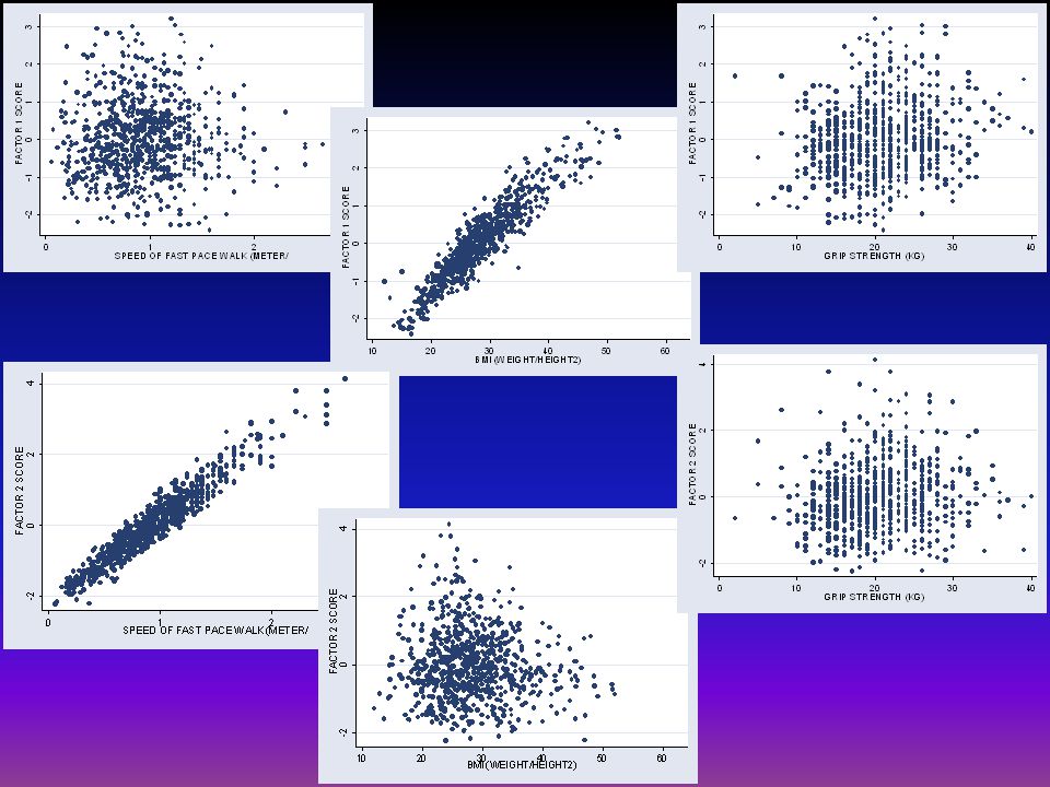
Here we can see that the factors are uncorrelated and the variable Exciting, Luxurious, Powerful, Stylish, and Fun are fairly strongly correlated with the first factor F1. The scatterplots of individual survey items do not show much as all items are on a 5-point Likert scale. In next slide we average the factor scores by car model and construct a scatterplot matrix of the average factors with points labeled by car model.

Example 2: McMaster’s FAD
Two underlying factors (m = 2) are suggested based on the eigenvalues. The two factor analysis gives loadings on the variables that contrast good trait vs. the bad family traits measured by the survey.

QUESTION Strongly Agree Agree Disagree Strongly Disagree 1. Planning family activities is difficult because we misunderstand each other. 1 2 3 4 2. In times of crisis we can turn to each other for support. 3. We cannot talk to each other about the sadness we feel. 4. Individuals are accepted for what they are. 5. We avoid discussing our fears and concerns. 6. We can express feelings to each other. 7. There are lots of bad feelings in the family. 8. We feel accepted for what we are. 9. Making decisions is a problem in our family. 10. We are able to make decisions about how to solve problems. 11. We do not get along well with each other. 12. We confide in each other

Warning: Very Mathematical!

Similar presentations

Presentation on theme: "Warning: Very Mathematical!"— Presentation transcript:

Similar presentations

About project

Feedback

Log in

Auth with social network:

Warning: Very Mathematical!

Similar presentations

Presentation on theme: "Warning: Very Mathematical!"— Presentation transcript:

Similar presentations

About project

Feedback