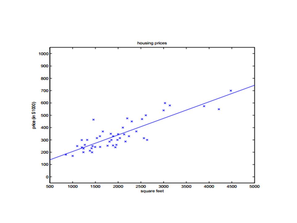
1. Linear Regression

2. Task: Learning a real valued function f: x->y where x=<x1,…,xn> as a linear function of the input features xi:
Using x0=1, we can write as:

3. Linear Regression 3 3

4. Cost function
We want to penalize from deviation from the target values:
Cost function J(q) is a convex quadratic function, so no local minima. 4 4

5. Linear Regression – Cost function5 5

6. Finding q that minimizes J(q)
Gradient descent:
Lets consider what happens for a single input pattern:

7. Gradient Descent
Stochastic Gradient Descent (update after each pattern) vs
Batch Gradient Descent (below):

8. Need for scaling input features8 8

10. Finding q that minimizes J(q)
Closed form solution:
where X is the row vector of data points.:

11. If we assume
with e(i) being iid and normally distributed around zero.
we can see that the least-squares regression corresponds to finding the maximum likelihood estimate of θ:

12. Underfitting: What if a line isn’t a good fit?
We can add more features => overfitting
 Regularization

13. Regularized Linear Regression13 13

14. Regularized Linear Regression14 14

15. Skipped Locally weighted linear regression You can read more in:

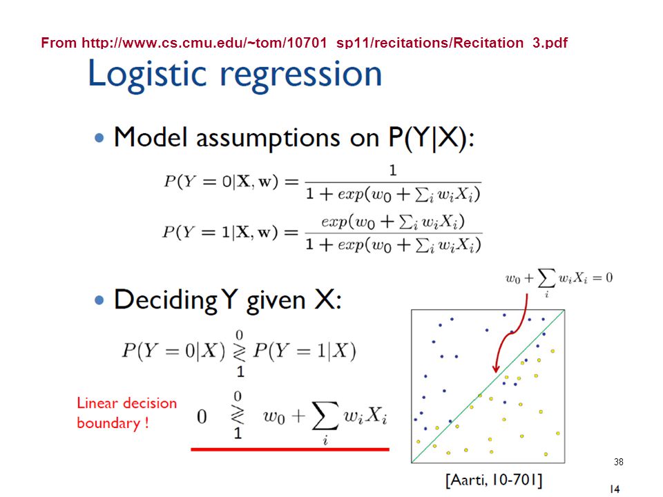
16. Logistic Regression

17. Logistic Regression - Motivation
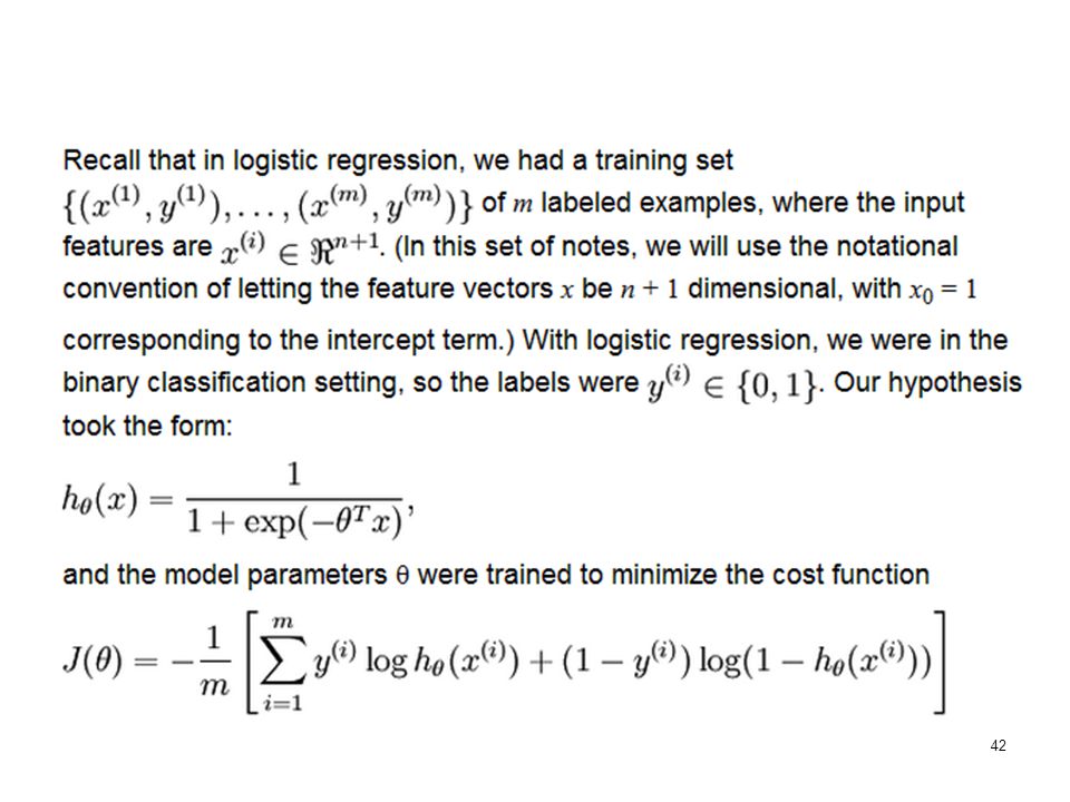
Lets now focus on the binary classification problem in which
y can take on only two values, 0 and 1.
x is a vector of real-valued features, < x1 … xn >
We could approach the classification problem ignoring the fact that y is discrete-valued, and use our old linear regression algorithm to try to predict y given x.
However, it is easy to construct examples where this method performs very poorly.
Intuitively, it also doesn’t make sense for h(x) to take values larger than 1 or smaller than 0 when we know that y ∈ {0, 1}.

18. Logistic Function 18 18

20. Derivative of the Logistic Function20 20

21. P(y | x; θ) = (h(x))y (1 − h(x))1−y
Interpretation:
hq(x) : estimate of probability that y=1 for a given x
hq(x) = P(y = 1 | x; θ)
Thus:
P(y = 1 | x; θ) = hq(x)
P(y = 0 | x; θ) = 1 − hq(x)
Which can be written more compactly as:
P(y | x; θ) = (h(x))y (1 − h(x))1−y 21 21

22. Logistic Regression 22 22

23. 23 23

24. 24 24

25. Mean Squared Error – Not Convex25 25

26. Alternative cost function?26 26

27. New cost function Make the cost function steeper:
Intuitively, saying that p(malignant|x)=0 and being wrong should be penalized severely! 27 27

28. New cost function 28 28

29. New cost function 29 29

30. 30 30

31. 31 31

32. 32 32

33. Minimizing the New Cost function
Convex! 33 33

34. Fitting q

35. Fitting q
Working with a single input and remembering h(x) = g(qTx):

36. Skipped
Alternative: Maximizing l(q) using Newton’s method

38. From http://www. cs. cmu. edu/~tom/10701_sp11/recitations/Recitation_338 38

39. Regularized Logistic Regression39 39

40. Multinomial Logistic Regression MaxEnt Classifier
Softmax Regression
Multinomial Logistic Regression
MaxEnt Classifier

41. Softmax Regression
Softmax regression model generalizes logistic regression to classification problems where the class label y can take on more than two possible values. 
The response variable y can take on any one of k values, so y ∈ {1, 2, , k}.

44. kx(n+1) matrix

45. 45 45

46. Softmax Derivation from Logistic Regression46 46

47. One fairly simple way to arrive at the multinomial logit model is to imagine, for K possible outcomes, running K-1 independent binary logistic regression models, in which one outcome is chosen as a "pivot" and then the other K-1 outcomes are separately regressed against the pivot outcome. This would proceed as follows, if outcome K (the last outcome) is chosen as the pivot:

48. 48 48

49. 49 49

50. Cost Function
We now describe the cost function that we'll use for softmax regression. In the equation below, 1{.} is the indicator function, so that 1{a true statement} = 1, and 1{a false statement} = 0. For example, 1{2 + 2 = 4} evaluates to 1; whereas 1{1 + 1 = 5} evaluates to 0.

51. Remember that for logistic regression, we had:
which can be written similarly as:

52. Note also that in softmax regression, we have that
The softmax cost function is similar, except that we now sum over the k different possible values of the class label.
Note also that in softmax regression, we have that 
: logistic
: softmax
                                       .

53. Fitting q

54. Over-parametrization
Softmax regression has an unusual property that it has a "redundant" set of parameters.
Suppose we take each of our parameter vectors θj, and subtract some fixed vector ψ from it, so that every θj is now replaced with θj − ψ (for every  ).
Our hypothesis now estimates the class label probabilities as

55. Over-parametrization
The softmax model is over-parameterized, meaning that for any hypothesis we might fit to the data, there are multiple parameter settings that give rise to exactly the same hypothesis function hθ mapping from inputs x to the predictions.
Further, if the cost function J(θ) is minimized by some setting of the parameters  ,
then it is also minimized by   
for any value of ψ.
                 ,

56. Weight Decay

57. Softmax function The softmax function will return:
a value close to 0 whenever xk is significantly less than the maximum of all the values,
a value close to 1 when applied to the maximum value, unless it is extremely close to the next-largest value.

58. which approximates the non-smooth function
Thus, the softmax function can be used to construct
a weighted average that behaves as a smooth function (which can be conveniently differentiated, etc.) and
which approximates the non-smooth function 

59. Logit 59 59

60. Let's say that the probability of success of some event is. 8
Let's say that the probability of success of some event is .8.  Then the probability of failure is = .2. 
The odds of success are defined as the ratio of the probability of success over the probability of failure. 
In the above example, the odds of success are .8/.2 = 4. 
That is to say that the odds of success are  4 to 1. 
The transformation from probability to odds is a monotonic transformation, meaning the odds increase as the probability increases or vice versa. 
Probability ranges from 0 and 1. 
Odds range from 0 and positive infinity. 

63. logit(p) = log(p/(1-p))= β0 + β1*x1 + ... + βk*xk
Why do we take all the trouble doing the transformation from probability to log odds?  One reason is that it is usually difficult to model a variable which has restricted range, such as probability.  This transformation is an attempt to get around the restricted range problem. 
It maps probability ranging between 0 and 1 to log odds ranging from negative infinity to positive infinity. 
Another reason is that among all of the infinitely many choices of transformation, the log of odds is one of the easiest to understand and interpret.  This transformation is called logit transformation.  The other common choice is the probit transformation, which will not be covered here.
A logistic regression model allows us to establish a relationship between a binary outcome variable and a group of predictor variables.  It models the logit-transformed probability as a linear relationship with the predictor variables. 
More formally, let y be the binary outcome variable indicating failure/success with 0/1 and p be the probability of y to be 1, p = prob(y=1). Let x1, .., xk be a set of predictor variables.  Then the logistic regression of y on x1, ..., xk estimates parameter values for β0, β1, , βk via maximum likelihood method of the following equation.
logit(p) = log(p/(1-p))= β0 + β1*x1  βk*xk
In terms of probabilities, the equation above is translated into
p= exp(β0 + β1*x1  βk*xk)/(1+exp(β0 + β1*x1  βk*xk))