1. What is a Network? Network = graph
Informally a graph is a set of nodes joined by a set of lines or arrows. 1 2 3 1 2 3 4 5 6 4 5 6

2. Graph-based representations
Representing a problem as a graph can provide a different point of view
Representing a problem as a graph can make a problem much simpler
More accurately, it can provide the appropriate tools for solving the problem

3. What is network theory?
Network theory provides a set of techniques for analysing graphs
Complex systems network theory provides techniques for analysing structure in a system of interacting agents, represented as a network
Applying network theory to a system means using a graph-theoretic representation

4. What makes a problem graph-like?
There are two components to a graph
Nodes and edges
In graph-like problems, these components have natural correspondences to problem elements
Entities are nodes and interactions between entities are edges
Most complex systems are graph-like

5. Friendship Network

6. Scientific collaboration network

7. Business ties in US
biotech-industry

8. Genetic interaction network

9. Protein-Protein Interaction Networks

10. Transportation Networks

11. Internet

12. Ecological Networks

13. Graph Theory - History
Leonhard Euler's paper on “Seven Bridges of Königsberg” ,
published in 1736.

14. Graph Theory - History Cycles in Polyhedra
Thomas P. Kirkman William R. Hamilton
Hamiltonian cycles in Platonic graphs

15. Graph Theory - History
Trees in Electric Circuits
Gustav Kirchhoff

16. Graph Theory - History
Enumeration of Chemical Isomers –n.b. topological distance a.k.a chemical distance
Arthur Cayley James J. Sylvester George Polya

17. Graph Theory - History Four Colors of Maps
Francis Guthrie Auguste DeMorgan

18. Definition: Graph G is an ordered triple G:=(V, E, f)
V is a set of nodes, points, or vertices.
E is a set, whose elements are known as edges or lines.
f is a function
maps each element of E
to an unordered pair of vertices in V.

19. Definitions Vertex Edge Basic Element Drawn as a node or a dot.
Vertex set of G is usually denoted by V(G), or V
Edge
A set of two elements
Drawn as a line connecting two vertices, called end vertices, or endpoints.
The edge set of G is usually denoted by E(G), or E.

20. Example
V:={1,2,3,4,5,6}
E:={{1,2},{1,5},{2,3},{2,5},{3,4},{4,5},{4,6}}

21. Simple Graphs
Simple graphs are graphs without multiple edges or self-loops.

22. Directed Graph (digraph)
Edges have directions
An edge is an ordered pair of nodes
loop
multiple arc
arc
node

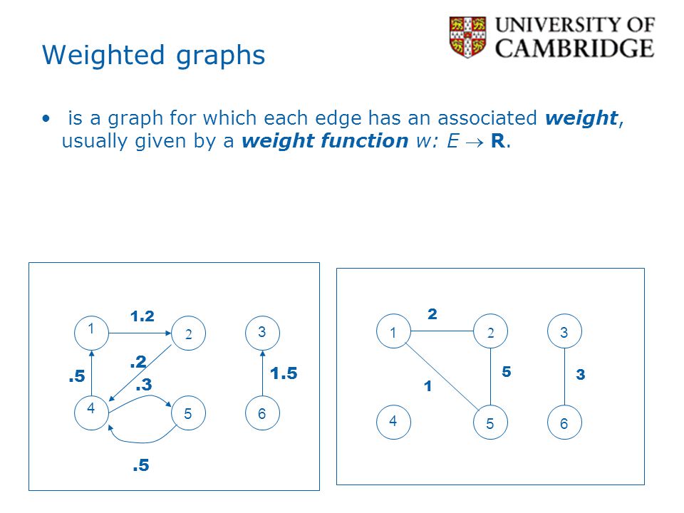
23. Weighted graphs
is a graph for which each edge has an associated weight, usually given by a weight function w: E  R. 1 2 3 4 5 6 .5
1.2 .2
1.5 .3

24. Structures and structural metrics
Graph structures are used to isolate interesting or important sections of a graph
Structural metrics provide a measurement of a structural property of a graph
Global metrics refer to a whole graph
Local metrics refer to a single node in a graph

25. Identify interesting sections of a graph
Graph structures
Identify interesting sections of a graph
Interesting because they form a significant domain-specific structure, or because they significantly contribute to graph properties
A subset of the nodes and edges in a graph that possess certain characteristics, or relate to each other in particular ways

26. Connectivity a graph is connected if
you can get from any node to any other by following a sequence of edges OR
any two nodes are connected by a path.
A directed graph is strongly connected if there is a directed path from any node to any other node.

27. Component
Every disconnected graph can be split up into a number of connected components.

28. Degree
Number of edges incident on a node
The degree of 5 is 3

29. Degree (Directed Graphs)
In-degree: Number of edges entering
Out-degree: Number of edges leaving
Degree = indeg + outdeg
outdeg(1)=2
indeg(1)=0
outdeg(2)=2
indeg(2)=2
outdeg(3)=1
indeg(3)=4

30. Degree: Simple Facts
If G is a graph with m edges, then  deg(v) = 2m = 2 |E |
If G is a digraph then  indeg(v)= outdeg(v) = |E |
Number of Odd degree Nodes is even

31. Walks A walk of length k in a graph is a succession of k
(not necessarily different) edges of the form
uv,vw,wx,…,yz.
This walk is denote by uvwx…xz, and is referred to
as a walk between u and z.
A walk is closed is u=z.

32. walk of length 5 CW of length 6 path of length 4
A path is a walk in which all the edges and all the nodes are different.
Walks and Paths
1,2,5,2,3, ,2,5,2,3,2, ,2,3,4,6
walk of length CW of length path of length 4

33. Cycle
A cycle is a closed walk in which all the edges are different.
1,2,5, ,3,4,5,2
3-cycle cycle

34. Special Types of Graphs
Empty Graph / Edgeless graph
No edge
Null graph
No nodes
Obviously no edge

35. Trees Connected Acyclic Graph
Two nodes have exactly one path between them c.f. routing, later

36. Special Trees
Paths
Stars

37. Regular
Connected Graph
All nodes have the same degree

38. Special Regular Graphs: Cycles
C C C5

39. Bipartite graph Shows up in coding&modulation algorithms
V can be partitioned into 2 sets V1 and V2 such that (u,v)E implies
either u V1 and v V2
OR v V1 and uV2.
Shows up in coding&modulation algorithms

40. Complete Graph Every pair of vertices are adjacent Has n(n-1)/2 edges
See switches&multicore interconnects

41. Complete Bipartite Graph
Bipartite Variation of Complete Graph
Every node of one set is connected to every other node on the other set
Stars

42. Planar Graphs Can be drawn on a plane such that no two edges intersect
K4 is the largest complete graph that is planar

43. Subgraph Vertex and edge sets are subsets of those of G
a supergraph of a graph G is a graph that contains G as a subgraph.

44. Special Subgraphs: Cliques
A clique is a maximum complete connected subgraph. A B D H F E C I G

45. Spanning subgraph Subgraph H has the same vertex set as G.
Possibly not all the edges
“H spans G”.

46. Spanning tree
Let G be a connected graph. Then a spanning tree in G is a subgraph of G that includes every node and is also a tree. Routing (esp bridges)

47. Isomorphism Bijection, i.e., a one-to-one mapping:
f : V(G) -> V(H)
u and v from G are adjacent if and only if f(u) and f(v) are adjacent in H.
If an isomorphism can be constructed between two graphs, then we say those graphs are isomorphic.

48. Isomorphism Problem Determining whether two graphs are isomorphic
Although these graphs look very different, they are isomorphic; one isomorphism between them is
f(a)=1 f(b)=6 f(c)=8 f(d)=3
f(g)=5 f(h)=2 f(i)=4 f(j)=7

49. Representation (Matrix)
Incidence Matrix
V x E
[vertex, edges] contains the edge's data
Adjacency Matrix
V x V
Boolean values (adjacent or not)
Or Edge Weights
What if matrix spare…?

50. Matrices

51. Representation (List)
Edge List
pairs (ordered if directed) of vertices
Optionally weight and other data
Adjacency List (node list)

52. Implementation of a Graph.
Adjacency-list representation
an array of |V | lists, one for each vertex in V.
For each u  V , ADJ [ u ] points to all its adjacent vertices.

53. Edge and Node Lists Node List Edge List 1 2 2 1 2 2 3 5 3 3 2 3 4 3 5
2 5
3 3
4 3
4 5
5 3
5 4
Node List
1 2 2
2 3 5
3 3
4 3 5
5 3 4

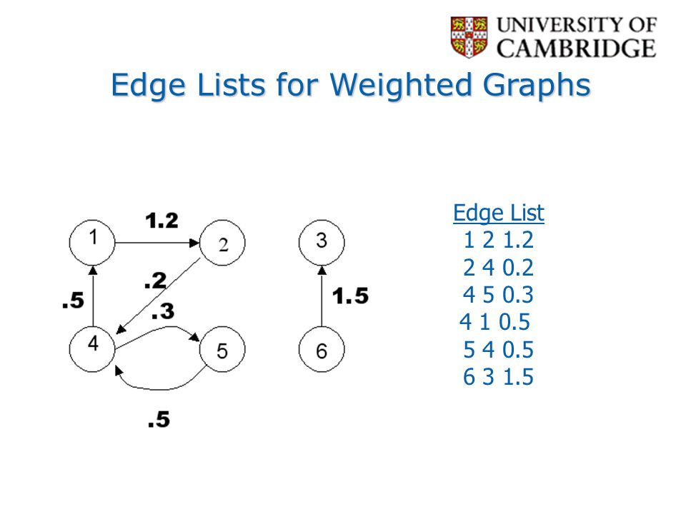
54. Edge Lists for Weighted Graphs

55. Topological Distance
A shortest path is the minimum path connecting two nodes.
The number of edges in the shortest path connecting p and q is the topological distance between these two nodes, dp,q

56. Distance Matrix
|V | x |V | matrix D = ( dij ) such that dij is the topological distance between i and j.

57. Random Graphs & Nature N nodes
Erdős and Renyi (1959)
p = 0.0 ; k = 0
N nodes
A pair of nodes has probability p of being connected.
Average degree, k ≈ pN
What interesting things can be said for different values of p or k ?
(that are true as N  ∞)
p = 0.09 ; k = 1
p = 1.0 ; k ≈ ½N2

58. Random Graphs Erdős and Renyi (1959) p = 0.0 ; k = 0 p = 0.09 ; k = 1
p = 1.0 ; k ≈ ½N2
Size of the largest connected cluster
Diameter (maximum path length between nodes) of the largest cluster
Average path length between nodes (if a path exists)

59. Random Graphs Erdős and Renyi (1959) p = 0.0 ; k = 0
p = 1.0 ; k ≈ ½N2
Size of largest component 1 5 11 12
Diameter of largest component 4 7 1
Average path length between nodes
0.0
2.0
4.2
1.0

60. Random Graphs Erdős and Renyi (1959) k phase transition
Percentage of nodes in largest component
Diameter of largest component (not to scale)
If k < 1:
small, isolated clusters
small diameters
short path lengths
At k = 1:
a giant component appears
diameter peaks
path lengths are high
For k > 1:
almost all nodes connected
diameter shrinks
path lengths shorten
1.0
This is similar to phase transitions in physics, when gases become liquids and liquids become solids.
(Even Bose-Einstein condensation is also relevant, it seems.)
1.0 k
phase transition

61. Random Graphs Erdős and Renyi (1959) What does this mean?
David
Mumford
Peter
Belhumeur
Kentaro
Toyama
Fan
Chung
Erdős and Renyi (1959)
What does this mean?
If connections between people can be modeled as a random graph, then…
Because the average person easily knows more than one person (k >> 1),
We live in a “small world” where within a few links, we are connected to anyone in the world.
Erdős and Renyi showed that average
path length between connected nodes is
The ln(N) expression is consistent with intuition about branching factors for trees. Even with lots of node repetition, if only 10% of each person’s contacts are not duplicates, links would rapidly span the entire population.
I know Peter from the computer vision community. Peter was a student of Mumford’s, I think. David Mumford is a Fields-Medal-winning mathematician, who has singlehandedly reduced the Erdos number of most computer vision researchers by doing work in computer vision. Fan Chung is a mathematician who has authored papers with both Erdos and Mumford.

62. BIG “IF”!!! Random Graphs Erdős and Renyi (1959) What does this mean?
David
Mumford
Peter
Belhumeur
Kentaro
Toyama
Fan
Chung
Erdős and Renyi (1959)
BIG “IF”!!!
What does this mean?
If connections between people can be modeled as a random graph, then…
Because the average person easily knows more than one person (k >> 1),
We live in a “small world” where within a few links, we are connected to anyone in the world.
Erdős and Renyi computed average
path length between connected nodes to be:

63. by MSR Redmond’s Social Computing Group
The Alpha Model
Watts (1999)
The people you know aren’t randomly chosen.
People tend to get to know those who are two links away (Rapoport *, 1957).
The real world exhibits a lot of clustering.
The Personal Map
by MSR Redmond’s Social Computing Group
* Same Anatol Rapoport, known for TIT FOR TAT!

64. The Alpha Model Watts (1999)
a model: Add edges to nodes, as in random graphs, but makes links more likely when two nodes have a common friend.
For a range of a values:
The world is small (average path length is short), and
Groups tend to form (high clustering coefficient).
Probability of linkage as a function
of number of mutual friends
(a is 0 in upper left,
1 in diagonal,
and ∞ in bottom right curves.)

65. The Alpha Model Watts (1999) a
a model: Add edges to nodes, as in random graphs, but makes links more likely when two nodes have a common friend.
For a range of a values:
The world is small (average path length is short), and
Groups tend to form (high clustering coefficient).
Clustering coefficient /
Normalized path length
Clustering coefficient (C) and
average path length (L)
plotted against a
Source: Duncan Watts, Six Degrees (2003). a

66. and a few distant people.
The Beta Model
Watts and Strogatz (1998)
b = 0
b = 0.125
b = 1
People know
their neighbors.
Clustered, but
not a “small world”
People know
their neighbors,
and a few distant people.
Clustered and
“small world”
People know
others at
random.
Not clustered,
but “small world”

67. The Beta Model Watts and Strogatz (1998)
Jonathan
Donner
Kentaro
Toyama
Watts and Strogatz (1998)
Nobuyuki
Hanaki
First five random links reduce the average path length of the network by half, regardless of N!
Both a and b models reproduce short- path results of random graphs, but also allow for clustering.
Small-world phenomena occur at threshold between order and chaos.
Clustering coefficient /
Normalized path length
Source: Duncan Watts, Six Degrees (2003).
Small-world phenomena of random graphs emerges even with less random links.
Jonathan Donner will be working with us at MSR India. Jonathan is now at the Earth Institute at Columbia, where he knows Nobuyuki Hanaki, who has co-authored papers with Duncan Watts.
Clustering coefficient (C) and average
path length (L) plotted against b

68. Power Laws Albert and Barabasi (1999)
What’s the degree (number of edges) distribution over a graph, for real- world graphs?
Random-graph model results in Poisson distribution.
But, many real-world networks exhibit a power-law distribution.
Source: Albert and Barabasi, “Statistical mechanics of complex networks.” Review of Modern Physics. 74: (2002)
Degree distribution of a random graph,
N = 10,000 p = k = 15.
(Curve is a Poisson curve, for comparison.)

69. Typical shape of a power-law distribution.
Power Laws
Albert and Barabasi (1999)
What’s the degree (number of edges) distribution over a graph, for real- world graphs?
Random-graph model results in Poisson distribution.
But, many real-world networks exhibit a power-law distribution.
Source: Duncan Watts, Six Degrees (2003).
Typical shape of a power-law distribution.

70. Power Laws Albert and Barabasi (1999)
Power-law distributions are straight lines in log-log space.
How should random graphs be generated to create a power-law distribution of node degrees?
Hint:
Pareto’s* Law: Wealth distribution follows a power law.
Source: Albert and Barabasi, “Statistical mechanics of complex networks.” Review of Modern Physics. 74: (2002)
Power laws in real networks:
(a) WWW hyperlinks
(b) co-starring in movies
(c) co-authorship of physicists
(d) co-authorship of neuroscientists
* Same Velfredo Pareto, who defined Pareto optimality in game theory.

71. “Map of the Internet” poster
Power Laws
Jennifer
Chayes
Anandan
Kentaro
Toyama
Albert and Barabasi (1999)
“The rich get richer!”
Power-law distribution of node distribution arises if
Number of nodes grow;
Edges are added in proportion to the number of edges a node already has.
Additional variable fitness coefficient allows for some nodes to grow faster than others.
“Map of the Internet” poster

72. Searchable Networks Kleinberg (2000)
Just because a short path exists, doesn’t mean you can easily find it.
You don’t know all of the people whom your friends know.
Under what conditions is a network searchable?

73. Searchable Networks Kleinberg (2000) Variation of Watts’s b model:
Lattice is d-dimensional (d=2).
One random link per node.
Parameter a controls probability of random link – greater for closer nodes.
b) For d=2, dip in time-to-search at a=2
For low a, random graph; no “geographic” correlation in links
For high a, not a small world; no short paths to be found.
Searchability dips at a=2, in simulation
Source: Jon Kleinberg, “Navigation in a small world.” Science, 406:845 (2000).

74. Searchable Networks Kleinberg (2000)
Ramin
Zabih
Kentaro
Toyama
Kleinberg (2000)
Watts, Dodds, Newman (2002) show that for d = 2 or 3, real networks are quite searchable.
Killworth and Bernard (1978) found that people tended to search their networks by d = 2: geography and profession.
Source: Duncan Watts, Six Degrees (2003).
I know Ramin as a computer vision researcher. Ramin is in the CS department at Cornell; I assume he knows Jon Kleinberg.
The Watts-Dodds-Newman model
closely fitting a real-world experiment

75. References
Aldous & Wilson, Graphs and Applications. An Introductory Approach, Springer, 2000.
WWasserman & Faust, Social Network Analysis, Cambridge University Press, 2008.