Constraint Satisfaction Problems

Constraint Satisfaction Problems
CS 271: Fall 2007 Instructor: Padhraic Smyth

Outline What is a CSP Backtracking for CSP Local search for CSPs
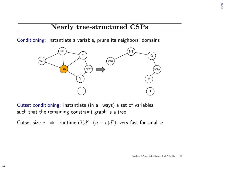
Problem structure and decomposition

Constraint Satisfaction Problems
What is a CSP? Finite set of variables V1, V2, …, Vn Nonempty domain of possible values for each variable DV1, DV2, … DVn Finite set of constraints C1, C2, …, Cm Each constraint Ci limits the values that variables can take, e.g., V1 ≠ V2 A state is defined as an assignment of values to some or all variables. Consistent assignment assignment does not violate the constraints CSP benefits Standard representation pattern Generic goal and successor functions Generic heuristics (no domain specific expertise).

CSPs (continued) An assignment is complete when every variable is mentioned. A solution to a CSP is a complete assignment that satisfies all constraints. Some CSPs require a solution that maximizes an objective function. Examples of Applications: Scheduling the time of observations on the Hubble Space Telescope Airline schedules Cryptography Computer vision -> image interpretation Scheduling your MS or PhD thesis exam 

CSP example: map coloring
Variables: WA, NT, Q, NSW, V, SA, T Domains: Di={red,green,blue} Constraints:adjacent regions must have different colors. E.g. WA  NT

CSP example: map coloring
Solutions are assignments satisfying all constraints, e.g. {WA=red,NT=green,Q=red,NSW=green,V=red,SA=blue,T=green}

Graph coloring More general problem than map coloring
Planar graph = graph in the 2d-plane with no edge crossings Guthrie’s conjecture (1852) Every planar graph can be colored with 4 colors or less Proved (using a computer) in 1977 (Appel and Haken)

Constraint graphs Constraint graph: nodes are variables
arcs are binary constraints Graph can be used to simplify search e.g. Tasmania is an independent subproblem (will return to graph structure later)

Varieties of CSPs Discrete variables Continuous variables
Finite domains; size d O(dn) complete assignments. E.g. Boolean CSPs: Boolean satisfiability (NP-complete). Infinite domains (integers, strings, etc.) E.g. job scheduling, variables are start/end days for each job Need a constraint language e.g StartJob1 +5 ≤ StartJob3. Infinitely many solutions Linear constraints: solvable Nonlinear: no general algorithm Continuous variables e.g. building an airline schedule or class schedule. Linear constraints solvable in polynomial time by LP methods.

Varieties of constraints
Unary constraints involve a single variable. e.g. SA  green Binary constraints involve pairs of variables. e.g. SA  WA Higher-order constraints involve 3 or more variables. Professors A, B,and C cannot be on a committee together Can always be represented by multiple binary constraints Preference (soft constraints) e.g. red is better than green often can be represented by a cost for each variable assignment combination of optimization with CSPs

CSP Example: Cryptharithmetic puzzle

CSP as a standard search problem
A CSP can easily be expressed as a standard search problem. Incremental formulation Initial State: the empty assignment {} Successor function: Assign a value to any unassigned variable provided that it does not violate a constraint Goal test: the current assignment is complete (by construction its consistent) Path cost: constant cost for every step (not really relevant) Can also use complete-state formulation Local search techniques (Chapter 4) tend to work well

CSP as a standard search problem
Solution is found at depth n (if there are n variables). Consider using BFS Branching factor b at the top level is nd At next level is (n-1)d …. end up with n!dn leaves even though there are only dn complete assignments!

Commutativity CSPs are commutative.
The order of any given set of actions has no effect on the outcome. Example: choose colors for Australian territories one at a time [WA=red then NT=green] same as [NT=green then WA=red] All CSP search algorithms can generate successors by considering assignments for only a single variable at each node in the search tree  there are dn leaves (will need to figure out later which variable to assign a value to at each node)

Backtracking search Similar to Depth-first search
Chooses values for one variable at a time and backtracks when a variable has no legal values left to assign. Uninformed algorithm No good general performance (see table p. 143)

Backtracking search function BACKTRACKING-SEARCH(csp) return a solution or failure return RECURSIVE-BACKTRACKING({} , csp) function RECURSIVE-BACKTRACKING(assignment, csp) return a solution or failure if assignment is complete then return assignment var  SELECT-UNASSIGNED-VARIABLE(VARIABLES[csp],assignment,csp) for each value in ORDER-DOMAIN-VALUES(var, assignment, csp) do if value is consistent with assignment according to CONSTRAINTS[csp] then add {var=value} to assignment result  RRECURSIVE-BACTRACKING(assignment, csp) if result  failure then return result remove {var=value} from assignment return failure

Backtracking example

Comparison of CSP algorithms on different problems
Median number of consistency checks over 5 runs to solve problem Parentheses -> no solution found USA: 4 coloring n-queens: n = 2 to 50 Zebra: see exercise 5.13

Improving CSP efficiency
Previous improvements on uninformed search  introduce heuristics For CSPS, general-purpose methods can give large gains in speed, e.g., Which variable should be assigned next? In what order should its values be tried? Can we detect inevitable failure early? Can we take advantage of problem structure? Note: CSPs are somewhat generic in their formulation, and so the heuristics are more general compared to methods in Chapter 4

Backtracking search function BACKTRACKING-SEARCH(csp) return a solution or failure return RECURSIVE-BACKTRACKING({} , csp) function RECURSIVE-BACKTRACKING(assignment, csp) return a solution or failure if assignment is complete then return assignment var  SELECT-UNASSIGNED-VARIABLE(VARIABLES[csp],assignment,csp) for each value in ORDER-DOMAIN-VALUES(var, assignment, csp) do if value is consistent with assignment according to CONSTRAINTS[csp] then add {var=value} to assignment result  RRECURSIVE-BACTRACKING(assignment, csp) if result  failure then return result remove {var=value} from assignment return failure

Minimum remaining values (MRV)
var  SELECT-UNASSIGNED-VARIABLE(VARIABLES[csp],assignment,csp) A.k.a. most constrained variable heuristic Heuristic Rule: choose variable with the fewest legal moves e.g., will immediately detect failure if X has no legal values

Degree heuristic for the initial variable
Heuristic Rule: select variable that is involved in the largest number of constraints on other unassigned variables. Degree heuristic can be useful as a tie breaker. In what order should a variable’s values be tried?

Least constraining value for value-ordering
Least constraining value heuristic Heuristic Rule: given a variable choose the least constraining value leaves the maximum flexibility for subsequent variable assignments

Forward checking Can we detect inevitable failure early?
And avoid it later? Forward checking idea: keep track of remaining legal values for unassigned variables. Terminate search when any variable has no legal values.

Forward checking Assign {WA=red}
Effects on other variables connected by constraints to WA NT can no longer be red SA can no longer be red

Forward checking Assign {Q=green}
Effects on other variables connected by constraints with WA NT can no longer be green NSW can no longer be green SA can no longer be green MRV heuristic would automatically select NT or SA next

Forward checking If V is assigned blue
Effects on other variables connected by constraints with WA NSW can no longer be blue SA is empty FC has detected that partial assignment is inconsistent with the constraints and backtracking can occur.

Example: 4-Queens Problem
{1,2,3,4} X3 X4 X2 1 3 2 4

{1,2,3,4} X3 { ,2, ,4} X4 { ,2,3, } X2 { , ,3,4} 1 3 2 4

{1,2,3,4} X3 { , , , } X4 { , ,3, } X2 { , ,3,4} 1 3 2 4

{1,2,3,4} X3 { ,2, ,4} X4 { ,2,3, } X2 { , , ,4} 1 3 2 4

{1,2,3,4} X3 { ,2, , } X4 { , ,3, } X2 { , , ,4} 1 3 2 4

{1,2,3,4} X3 { ,2, , } X4 { , , , } X2 { , ,3,4} 1 3 2 4

Problem b a c e d Consider the constraint graph on the right.
The domain for every variable is [1,2,3,4]. There are 2 unary constraints: - variable “a” cannot take values 3 and 4. variable “b” cannot take value 4. There are 8 binary constraints stating that variables connected by an edge cannot have the same value. Find a solution for this CSP by using the following heuristics: minimum value heuristic, degree heuristic, forward checking. b a c e d

Problem MVH a=1 (for example) FC+MVH b=2 FC+MVH+DH c=3 FC+MVH d=4
Consider the constraint graph on the right. The domain for every variable is [1,2,3,4]. There are 2 unary constraints: - variable “a” cannot take values 3 and 4. variable “b” cannot take value 4. There are 8 binary constraints stating that variables connected by an edge cannot have the same value. Find a solution for this CSP by using the following heuristics: minimum value heuristic, degree heuristic, forward checking. MVH a=1 (for example) FC+MVH b=2 FC+MVH+DH c=3 FC+MVH d=4 FC e=1 b a c e d

Constraint propagation
Solving CSPs with combination of heuristics plus forward checking is more efficient than either approach alone FC checking does not detect all failures. E.g., NT and SA cannot be blue

Constraint propagation
Techniques like CP and FC are in effect eliminating parts of the search space Somewhat complementary to search Constraint propagation goes further than FC by repeatedly enforcing constraints locally Needs to be faster than actually searching to be effective Arc-consistency (AC) is a systematic procedure for constraing propagation

Arc consistency An Arc X  Y is consistent if
for every value x of X there is some value y consistent with x (note that this is a directed property) Consider state of search after WA and Q are assigned: SA  NSW is consistent if SA=blue and NSW=red

Arc consistency X  Y is consistent if
for every value x of X there is some value y consistent with x NSW  SA is consistent if NSW=red and SA=blue NSW=blue and SA=???

Arc consistency Can enforce arc-consistency:
Arc can be made consistent by removing blue from NSW Continue to propagate constraints…. Check V  NSW Not consistent for V = red Remove red from V

Arc consistency Continue to propagate constraints….
SA  NT is not consistent and cannot be made consistent Arc consistency detects failure earlier than FC

Arc consistency checking
Can be run as a preprocessor or after each assignment Or as preprocessing before search starts AC must be run repeatedly until no inconsistency remains Trade-off Requires some overhead to do, but generally more effective than direct search In effect it can eliminate large (inconsistent) parts of the state space more effectively than search can Need a systematic method for arc-checking If X loses a value, neighbors of X need to be rechecked: i.e. incoming arcs can become inconsistent again (outgoing arcs will stay consistent).

Arc consistency algorithm (AC-3)
function AC-3(csp) return the CSP, possibly with reduced domains inputs: csp, a binary csp with variables {X1, X2, …, Xn} local variables: queue, a queue of arcs initially the arcs in csp while queue is not empty do (Xi, Xj)  REMOVE-FIRST(queue) if REMOVE-INCONSISTENT-VALUES(Xi, Xj) then for each Xk in NEIGHBORS[Xi ] do add (Xi, Xj) to queue function REMOVE-INCONSISTENT-VALUES(Xi, Xj) return true iff we remove a value removed  false for each x in DOMAIN[Xi] do if no value y in DOMAIN[Xi] allows (x,y) to satisfy the constraints between Xi and Xj then delete x from DOMAIN[Xi]; removed  true return removed (from Mackworth, 1977)

Another problem to try [R,B,G] [R,B,G] [R] [R,B,G] [R,B,G]
Use all heuristics including arc-propagation to solve this problem.

Complexity of AC-3 A binary CSP has at most n2 arcs
Each arc can be inserted in the queue d times (worst case) (X, Y): only d values of X to delete Consistency of an arc can be checked in O(d2) time Complexity is O(n2 d3)

Arc-consistency as message-passing
This is a propagation algorithm. It’s like sending messages to neighbors on the graph. How do we schedule these messages? Every time a domain changes, all incoming messages need to be re-sent. Repeat until convergence  no message will change any domains. Since we only remove values from domains when they can never be part of a solution, an empty domain means no solution possible at all  back out of that branch. Forward checking is simply sending messages into a variable that just got its value assigned. First step of arc-consistency.

K-consistency Arc consistency does not detect all inconsistencies:
Partial assignment {WA=red, NSW=red} is inconsistent. Stronger forms of propagation can be defined using the notion of k-consistency. A CSP is k-consistent if for any set of k-1 variables and for any consistent assignment to those variables, a consistent value can always be assigned to any kth variable. E.g. 1-consistency = node-consistency E.g. 2-consistency = arc-consistency E.g. 3-consistency = path-consistency Strongly k-consistent: k-consistent for all values {k, k-1, …2, 1}

Trade-offs Running stronger consistency checks… Takes more time
But will reduce branching factor and detect more inconsistent partial assignments No “free lunch” In worst case n-consistency takes exponential time

Further improvements Checking special constraints
Checking Alldif(…) constraint E.g. {WA=red, NSW=red} Checking Atmost(…) constraint Bounds propagation for larger value domains Intelligent backtracking Standard form is chronological backtracking i.e. try different value for preceding variable. More intelligent, backtrack to conflict set. Set of variables that caused the failure or set of previously assigned variables that are connected to X by constraints. Backjumping moves back to most recent element of the conflict set. Forward checking can be used to determine conflict set.

Local search for CSPs Use complete-state representation For CSPs
Initial state = all variables assigned values Successor states = change 1 (or more) values For CSPs allow states with unsatisfied constraints (unlike backtracking) operators reassign variable values hill-climbing with n-queens is an example Variable selection: randomly select any conflicted variable Value selection: min-conflicts heuristic Select new value that results in a minimum number of conflicts with the other variables

Local search for CSP function MIN-CONFLICTS(csp, max_steps) return solution or failure inputs: csp, a constraint satisfaction problem max_steps, the number of steps allowed before giving up current  an initial complete assignment for csp for i = 1 to max_steps do if current is a solution for csp then return current var  a randomly chosen, conflicted variable from VARIABLES[csp] value  the value v for var that minimize CONFLICTS(var,v,current,csp) set var = value in current return failure

Min-conflicts example 1
h=5 h=3 h=1 Use of min-conflicts heuristic in hill-climbing.

Min-conflicts example 2
A two-step solution for an 8-queens problem using min-conflicts heuristic At each stage a queen is chosen for reassignment in its column The algorithm moves the queen to the min-conflict square breaking ties randomly.

Advantages of local search
Local search can be particularly useful in an online setting Airline schedule example E.g., mechanical problems require than 1 plane is taken out of service Can locally search for another “close” solution in state-space Much better (and faster) in practice than finding an entirely new schedule The runtime of min-conflicts is roughly independent of problem size. Can solve the millions-queen problem in roughly 50 steps. Why? n-queens is easy for local search because of the relatively high density of solutions in state-space

Graph structure and problem complexity
Solving disconnected subproblems Suppose each subproblem has c variables out of a total of n. Worst case solution cost is O(n/c dc), i.e. linear in n Instead of O(d n), exponential in n E.g. n= 80, c= 20, d=2 280 = 4 billion years at 1 million nodes/sec. 4 * 220= .4 second at 1 million nodes/sec

Tree-structured CSPs Theorem:
if a constraint graph has no loops then the CSP can be solved in O(nd 2) time linear in the number of variables! Compare difference with general CSP, where worst case is O(d n)

Algorithm for Solving Tree-structured CSPs
Choose some variable as root, order variables from root to leaves such that every node’s parent precedes it in the ordering. Label variables from X1 to Xn) Every variable now has 1 parent Backward Pass For j from n down to 2, apply arc consistency to arc [Parent(Xj), Xj) ] Remove values from Parent(Xj) if needed Forward Pass For j from 1 to n assign Xj consistently with Parent(Xj )

Tree CSP Example G B

Tree CSP Example Backward Pass (constraint propagation) B R G B R G B

Tree CSP Example Backward Pass (constraint propagation) Forward Pass
(assignment) B G R R G B

Tree CSP complexity Overall complexity is O(nd 2)
Backward pass n arc checks Each has complexity d2 at worst Forward pass n variable assignments, O(nd) Overall complexity is O(nd 2) Algorithm works because if the backward pass succeeds, then every variable by definition has a legal assignment in the forward pass

What about non-tree CSPs?
General idea is to convert the graph to a tree 2 general approaches Assign values to specific variables (Cycle Cutset method) Construct a tree-decomposition of the graph - Connected subproblems (subgraphs) form a tree structure

Cycle-cutset conditioning
Choose a subset S of variables from the graph so that graph without S is a tree S = “cycle cutset” For each possible consistent assignment for S Remove any inconsistent values from remaining variables that are inconsistent with S Use tree-structured CSP to solve the remaining tree-structure If it has a solution, return it along with S If not, continue to try other assignments for S

Finding the optimal cutset
If c is small, this technique works very well However, finding smallest cycle cutset is NP-hard But there are good approximation algorithms

Tree Decompositions

Rules for a Tree Decomposition
Every variable appears in at least one of the subproblems If two variables are connected in the original problem, they must appear together (with the constraint) in at least one subproblem If a variable appears in two subproblems, it must appear in each node on the path.

Tree Decomposition Algorithm
View each subproblem as a “super-variable” Domain = set of solutions for the subproblem Obtained by running a CSP on each subproblem E.g., 6 solutions for 3 fully connected variables in map problem Now use the tree CSP algorithm to solve the constraints connecting the subproblems Declare a subproblem a root node, create tree Backward and forward passes Example of “divide and conquer” strategy

Complexity of Tree Decomposition
Many possible tree decompositions for a graph Tree-width of a tree decomposition = 1 less than the size of the largest subproblem Tree-width of a graph = minimum tree width If a graph has tree width w, then solving the CSP can be done in O(n dw+1) time (why?) CSPs of bounded tree-width are solvable in polynomial time Finding the optimal tree-width of a graph is NP-hard, but good heuristics exist.

Summary CSPs special kind of problem: states defined by values of a fixed set of variables, goal test defined by constraints on variable values Backtracking=depth-first search with one variable assigned per node Heuristics Variable ordering and value selection heuristics help significantly Constraint propagation does additional work to constrain values and detect inconsistencies Works effectively when combined with heuristics Iterative min-conflicts is often effective in practice. Graph structure of CSPs determines problem complexity e.g., tree structured CSPs can be solved in linear time.

Constraint Satisfaction Problems

Similar presentations

Presentation on theme: "Constraint Satisfaction Problems"— Presentation transcript:

Similar presentations

About project

Feedback

Log in

Auth with social network:

Constraint Satisfaction Problems

Similar presentations

Presentation on theme: "Constraint Satisfaction Problems"— Presentation transcript:

Similar presentations

About project

Feedback