1. Lecture notes #8: empirical studies of convergence

2. Facts: The gap between rich and poor countries is large
It is rather persistent
Standard neo-classical models would predict rather rapid convergence

3. Productivity growth seems to accelerate over time

4. The gap between rich and poor countries is huge:

5. Can we explain it?

6. It does not add up Common estimates suggest α = 1/3
Therefore, to have a 10-fold difference in GDP, we need a 20-fold difference in savings rate (2 % vs. 40 %)
More leeway if technology differed across countries, but unlikely if technology is transferable
So what do we do?

7. If α were greater? Growth would take more time to fall to zero
Convergence would be slower
The speed of convergence is the coefficient of gdp growth on (local) initial log gdp
Income differences between countries would be magnified

8. Computing the speed of convergence

9. An extreme case: α = 1,g=0 The speed of convergence goes to zero
The convergence path becomes a balanced growth path at a constant rate
MRK no longer falling  capital accumulation can sustain long-run growth
The growth rate is now endogenous and depends on preferences

10. Convergence in neo-classical models
Neo-Classical models: each country converges to its own steady state
All own steady states grow at the same rate
But the level depend on policies, savings rates, etc
Similar countries converge to same GDP per capita

11. Convergence in endogenous growth models
A laggard never closes the gap
Therefore, no convergence in income levels
This because MPK is no higher for the laggard
Furthermore, differences in policies affect the long-run growth rate

12. Looking at convergence allows us to
Test the relevance of endogenous growth models
Assess the magnitude of the returns to accumulable factors

13. Two approaches
Barro and Sala-i-Martin: take a data set of similar economic units and look at convergence between them in pc GDP
Mankiw-Romer-Weil: take a cross-country regression of growth rates on initial income controlling for own long-run steady state

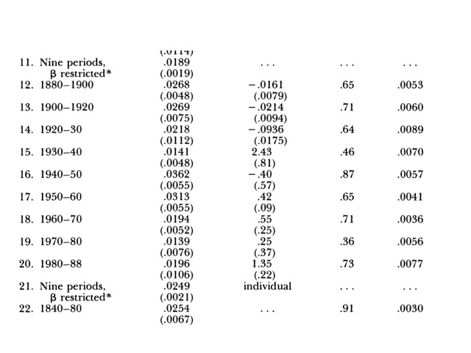
14. Barro and Sala-i-Martin
They use a data-base of U.S. states over a long-run period
They estimate the equivalent of our local speed of convergence regression:

18. The BSM Universal Law of Convergence:
The speed of convergence is 2 % per year

19. What do we expect? The Solow model predicts (δ+g)(1-α)
A reasonable calibration is δ=0.06, g=0.02, α=0.3
This gives v=5.6 % per year

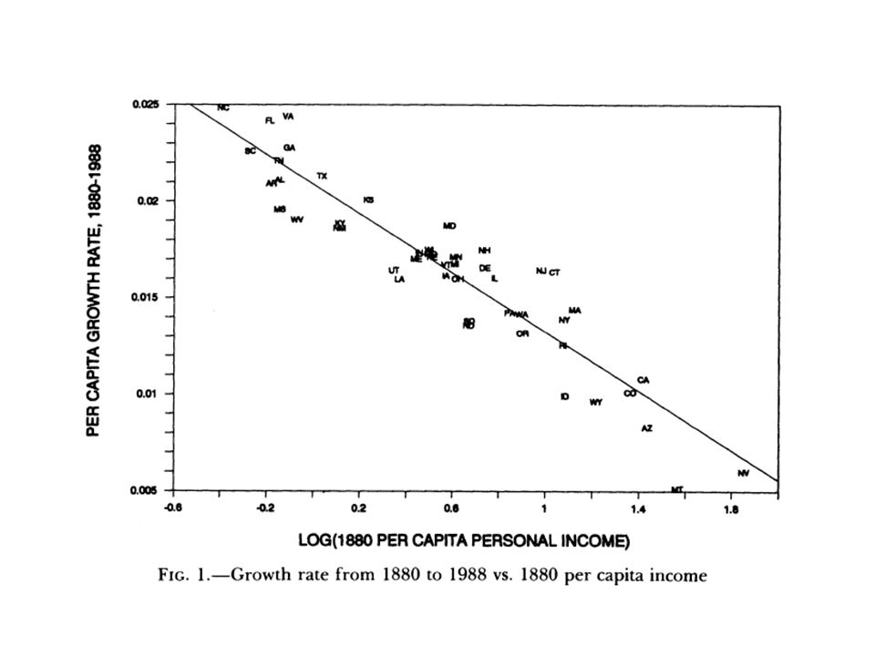
20. How universal is the law?

22. Findings:
The more similar the countries, the more it holds unconditionally
The less similar the countries, the more likely we find divergence
But the law is restored if controls are added, controlling for own steady state

23. How to eradicate poverty?
1. Adopt the policies and institutions of advanced countries
2. Wait!
How long? Suppose I am 10 times poorer than the US. How long does it take to be 2 times poorer?

25. What do we get? With v=0.02, ρ0 = 0.1, ρ1 = 0.5,
 t = 60 years!
With v=0.056, we instead get
t = 21 years
We want to understand why the speed of convergence is so low
Can policy increase the speed of convergence?

26. Gloom?
In principle, the speed of convergence only depends on the deep technological parameters
That it is low tells us that the technology is not what we thought it was
But it does not tell us we can increase v

27. Mankiw-Romer and Weil
National accounts suggest that the elasticity of capital is 0.3
Speed of convergence is more like
1-v/(g+δ) = /0.08 = 0.75
To reconcile these two facts, they introduce another form of capital: Human capital

28. The Augmented Solow model

29. The balanced-growth path

30. Explaining cross-country differenced in pcGDP:
The preceding equations define “own” steady state
They use it to see if it explains cross-country income differences:

31. Measuring sH

33. What have we learned?
We have seen that with α = 0.3, it is difficult to explain X-country income differences
But now what matters is α + β, which acts as α
So with α + β large enough we can explain cross-country differences.
A natural question is: can we also expect slow convergence?

34. Recomputing the speed of convergence

35. Empirical strategy
Investment rates and schooling are kept to proxy for own steady state
Initial output is added
Coefficient in initial output related to SOV as in BSM
No other control variable is added in strict interpretation of Solow model

36. Old Solow does not work…

37. …but new does.

38. Does it add up?

39. Summary
The Solow model predicts too low income disparities and too quick convergence
The AK model predicts zero convergence and widening disparities
The Augmented Solow model does well to predict both the disparities and the speed of convergence