Download presentation
Presentation is loading. Please wait.

1
418382 สภาพแวดล้อมการทำงานคอมพิวเตอร์กราฟิกส์ การบรรยายครั้งที่ 7

22
CS 445 / 645 Introduction to Computer Graphics
Lecture 22 Hermite Splines

23
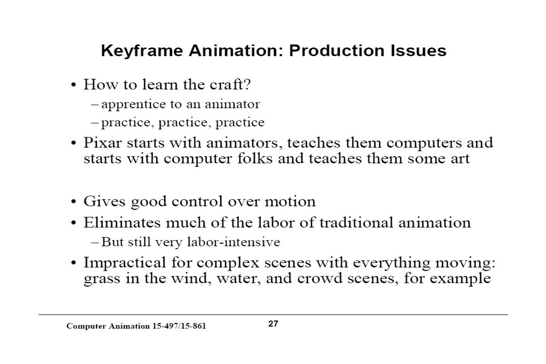
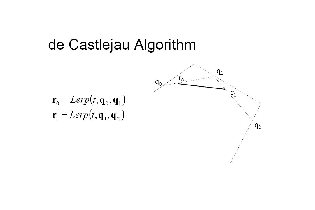
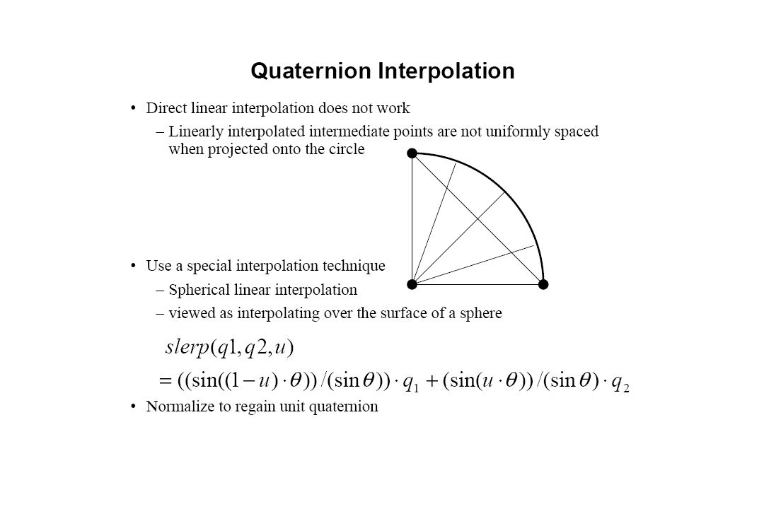
Splines – Old School Duck Spline

24
Representations of Curves
Use a sequence of points… Piecewise linear - does not accurately model a smooth line Tedious to create list of points Expensive to manipulate curve because all points must be repositioned Instead, model curve as piecewise-polynomial x = x(t), y = y(t), z = z(t) where x(), y(), z() are polynomials
, y = y(t), z = z(t) where x(), y(), z() are polynomials.")
25
Specifying Curves (hyperlink)
Control Points A set of points that influence the curve’s shape Knots Control points that lie on the curve Interpolating Splines Curves that pass through the control points (knots) Approximating Splines Control points merely influence shape
 Approximating Splines. Control points merely influence shape.")
26
Parametric Curves Very flexible representation
They are not required to be functions They can be multivalued with respect to any dimension

27
Cubic Polynomials x(t) = axt3 + bxt2 + cxt + dx
Similarly for y(t) and z(t) Let t: (0 <= t <= 1) Let T = [t3 t2 t 1] Coefficient Matrix C Curve: Q(t) = T*C
 and z(t) Let t: (0 <= t <= 1) Let T = [t3 t2 t 1] Coefficient Matrix C. Curve: Q(t) = T*C.")
28
Piecewise Curve Segments
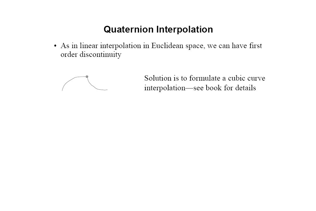
One curve constructed by connecting many smaller segments end-to-end Must have rules for how the segments are joined Continuity describes the joint Parametric continuity Geometric continuity

29
Parametric Continuity
C1 is tangent continuity (velocity) C2 is 2nd derivative continuity (acceleration) Matching direction and magnitude of dn / dtn Cn continous
 C2 is 2nd derivative continuity (acceleration) Matching direction and magnitude of dn / dtn. Cn continous.")
30
Geometric Continuity If positions match
G0 geometric continuity If direction (but not necessarily magnitude) of tangent matches G1 geometric continuity The tangent value at the end of one curve is proportional to the tangent value of the beginning of the next curve
 of tangent matches. G1 geometric continuity. The tangent value at the end of one curve is proportional to the tangent value of the beginning of the next curve.")
31
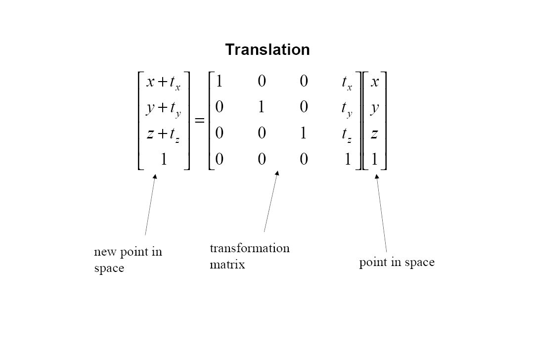
Parametric Cubic Curves
In order to assure C2 continuity, curves must be of at least degree 3 Here is the parametric definition of a cubic (degree 3) spline in two dimensions How do we extend it to three dimensions?
 spline in two dimensions. How do we extend it to three dimensions")
32
Parametric Cubic Splines
Can represent this as a matrix too

33
Coefficients So how do we select the coefficients?
[ax bx cx dx] and [ay by cy dy] must satisfy the constraints defined by the knots and the continuity conditions

34
Parametric Curves Difficult to conceptualize curve as x(t) = axt3 + bxt2 + cxt + dx (artists don’t think in terms of coefficients of cubics) Instead, define curve as weighted combination of 4 well- defined cubic polynomials (wait a second! Artists don’t think this way either!) Each curve type defines different cubic polynomials and weighting schemes
 Each curve type defines different cubic polynomials and weighting schemes.")
35
Parametric Curves Hermite – two endpoints and two endpoint tangent vectors Bezier - two endpoints and two other points that define the endpoint tangent vectors Splines – four control points C1 and C2 continuity at the join points Come close to their control points, but not guaranteed to touch them Examples of Splines

36
Hermite Cubic Splines An example of knot and continuity constraints

37
Hermite Cubic Splines One cubic curve for each dimension
A curve constrained to x/y-plane has two curves:

38
Hermite Cubic Splines A 2-D Hermite Cubic Spline is defined by eight parameters: a, b, c, d, e, f, g, h How do we convert the intuitive endpoint constraints into these (relatively) unintuitive eight parameters? We know: (x, y) position at t = 0, p1 (x, y) position at t = 1, p2 (x, y) derivative at t = 0, dp/dt (x, y) derivative at t = 1, dp/dt
 unintuitive eight parameters We know: (x, y) position at t = 0, p1. (x, y) position at t = 1, p2. (x, y) derivative at t = 0, dp/dt. (x, y) derivative at t = 1, dp/dt.")
39
Hermite Cubic Spline We know: (x, y) position at t = 0, p1
 position at t = 0, p1")
40
Hermite Cubic Spline We know: (x, y) position at t = 1, p2
 position at t = 1, p2")
41
Hermite Cubic Splines So far we have four equations, but we have eight unknowns Use the derivatives

42
Hermite Cubic Spline We know: (x, y) derivative at t = 0, dp/dt
 derivative at t = 0, dp/dt")
43
Hermite Cubic Spline We know: (x, y) derivative at t = 1, dp/dt
 derivative at t = 1, dp/dt")
44
Hermite Specification
Matrix equation for Hermite Curve t t t t0 t = 0 p1 t = 1 p2 t = 0 r p1 r p2 t = 1

45
Solve Hermite Matrix

46
Spline and Geometry Matrices
MHermite GHermite

47
Resulting Hermite Spline Equation

48
Sample Hermite Curves

49
Blending Functions By multiplying first two matrices in lower-left equation, you have four functions of ‘t’ that blend the four control parameters These are blending functions

50
Hermite Blending Functions
If you plot the blending functions on the parameter ‘t’

51
Hermite Blending Functions
Remember, each blending function reflects influence of P1, P2, DP1, DP2 on spline’s shape

52
CS 445 / 645 Introduction to Computer Graphics
Lecture 23 Bézier Curves

53
Splines - History Draftsman use ‘ducks’ and strips of wood (splines) to draw curves Wood splines have second- order continuity And pass through the control points A Duck (weight) Ducks trace out curve
 Ducks trace out curve.")
54
Bézier Curves Similar to Hermite, but more intuitive definition of endpoint derivatives Four control points, two of which are knots

55
Bézier Curves The derivative values of the Bezier Curve at the knots are dependent on the adjacent points The scalar 3 was selected just for this curve

56
Bézier vs. Hermite We can write our Bezier in terms of Hermite
Note this is just matrix form of previous equations

57
Bézier vs. Hermite Now substitute this in for previous Hermite MBezier

58
Bézier Basis and Geometry Matrices
Matrix Form But why is MBezier a good basis matrix?

59
Bézier Blending Functions
Look at the blending functions This family of polynomials is called order-3 Bernstein Polynomials C(3, k) tk (1-t)3-k; 0<= k <= 3 They are all positive in interval [0,1] Their sum is equal to 1
 tk (1-t)3-k; 0<= k <= 3. They are all positive in interval [0,1] Their sum is equal to 1.")
60
Bézier Blending Functions
Thus, every point on curve is linear combination of the control points The weights of the combination are all positive The sum of the weights is 1 Therefore, the curve is a convex combination of the control points

61
Convex combination of control points
Will always remain within bounding region (convex hull) defined by control points
 defined by control points.")
66
Why more spline slides? Bezier and Hermite splines have global influence One could create a Bezier curve that required 15 points to define the curve… Moving any one control point would affect the entire curve Piecewise Bezier or Hermite don’t suffer from this, but they don’t enforce derivative continuity at join points B-splines consist of curve segments whose polynomial coefficients depend on just a few control points Local control Examples of Splines

67
B-Spline Curve (cubic periodic)
Start with a sequence of control points Select four from middle of sequence (pi-2, pi-1, pi, pi+1) d Bezier and Hermite goes between pi-2 and pi+1 B-Spline doesn’t interpolate (touch) any of them but approximates going through pi-1 and pi p2 p 6 p1 Q4 t4 Q5 t5 Q3 t6 Q6 p3 t3 t7 p0 p 4 p 5
 d. Bezier and Hermite goes between pi-2 and pi+1. B-Spline doesn’t interpolate (touch) any of them but approximates going through pi-1 and pi. p2. p 6. p1. Q4. t4. Q5. t5. Q3. t6. Q6. p3. t3. t7. p0. p 4. p 5.")
68
Uniform B-Splines Approximating Splines
Approximates n+1 control points P0, P1, …, Pn, n ¸ 3 Curve consists of n –2 cubic polynomial segments Q3, Q4, … Qn t varies along B-spline as Qi: ti <= t < ti+1 ti (i = integer) are knot points that join segment Qi to Qi+1 Curve is uniform because knots are spaced at equal intervals of parameter, t
 are knot points that join segment Qi to Qi+1. Curve is uniform because knots are spaced at equal intervals of parameter, t.")
69
Uniform B-Splines First curve segment, Q3, is defined by first four control points Last curve segment, Qm, is defined by last four control points, Pm-3, Pm-2, Pm-1, Pm Each control point affects four curve segments

70
B-spline Basis Matrix Formulate 16 equations to solve the 16 unknowns
The 16 equations enforce the C0, C1, and C2 continuity between adjoining segments, Q

71
B-Spline Points along B-Spline are computed just as with Bezier Curves

72
B-Spline By far the most popular spline used C0, C1, and C2 continuous

73
Nonuniform, Rational B-Splines (NURBS)
The native geometry element in Maya Models are composed of surfaces defined by NURBS, not polygons NURBS are smooth NURBS require effort to make non-smooth

74
Converting Between Splines
Consider two spline basis formulations for two spline types

75
Converting Between Splines
We can transform the control points from one spline basis to another

76
Converting Between Splines
With this conversion, we can convert a B-Spline into a Bezier Spline Bezier Splines are easy to render

77
Rendering Splines Horner’s Method
Incremental (Forward Difference) Method Subdivision Methods
 Method. Subdivision Methods.")
78
Horner’s Method Three multiplications Three additions

79
Forward Difference But this still is expensive to compute
Solve for change at k (Dk) and change at k+1 (Dk+1) Boot strap with initial values for x0, D0, and D1 Compute x3 by adding x0 + D0 + D1
 and change at k+1 (Dk+1) Boot strap with initial values for x0, D0, and D1. Compute x3 by adding x0 + D0 + D1.")
80
Subdivision Methods Bezier

81
Rendering Bezier Spline
public void spline(ControlPoint p0, ControlPoint p1, ControlPoint p2, ControlPoint p3, int pix) { float len = ControlPoint.dist(p0,p1) + ControlPoint.dist(p1,p2) + ControlPoint.dist(p2,p3); float chord = ControlPoint.dist(p0,p3); if (Math.abs(len - chord) < 0.25f) return; fatPixel(pix, p0.x, p0.y); ControlPoint p11 = ControlPoint.midpoint(p0, p1); ControlPoint tmp = ControlPoint.midpoint(p1, p2); ControlPoint p12 = ControlPoint.midpoint(p11, tmp); ControlPoint p22 = ControlPoint.midpoint(p2, p3); ControlPoint p21 = ControlPoint.midpoint(p22, tmp); ControlPoint p20 = ControlPoint.midpoint(p12, p21); spline(p20, p12, p11, p0, pix); spline(p3, p22, p21, p20, pix); }
 { float len = ControlPoint.dist(p0,p1) + ControlPoint.dist(p1,p2) + ControlPoint.dist(p2,p3); float chord = ControlPoint.dist(p0,p3); if (Math.abs(len - chord) < 0.25f) return; fatPixel(pix, p0.x, p0.y); ControlPoint p11 = ControlPoint.midpoint(p0, p1); ControlPoint tmp = ControlPoint.midpoint(p1, p2); ControlPoint p12 = ControlPoint.midpoint(p11, tmp); ControlPoint p22 = ControlPoint.midpoint(p2, p3); ControlPoint p21 = ControlPoint.midpoint(p22, tmp); ControlPoint p20 = ControlPoint.midpoint(p12, p21); spline(p20, p12, p11, p0, pix); spline(p3, p22, p21, p20, pix); }")
117
ควอเทอเนียน ควอเทอเนียนที่แทนการหมุนเป็นมุม รอบแกน (x,y,z) คือ
 คือ")
118
ตัวอย่าง จงหาควอเทอเนียนที่แทนการหมุนเป็นมุม 60 องศารอบแกน (1,1,1)
เวกเตอร์หนึ่งหน่วยของแกนคือ คำนวณค่า cos และ sin และจะได้ว่าควอเทอเนียนคือ

119
ตัวอย่าง ควอเทอเนียนต่อไปนี้แทนการหมุนกี่องศา รอบแกนอะไร? เราได้ว่า
ฉะนั้น แกนที่หมุนรอบคือ

120
การคูณควอเทอเนียน หลีกเลี่ยงการคูณควอเทอเนียนตรงๆ
เพราะการคำนวณยุ่งยากและมีสิทธิ์ผิดมาก ใช้ความเข้าใจความหมายของควอเทอเนียนทำการคำนวณดีกว่า

121
ตัวอย่าง ให้ จงคำนวณ

122
ตัวอย่าง q1 คือการหมุนเป็นมุม 90 องศา รอบแกน (3/5, 0, 4/5)
ฉะนั้น q1q2 คือการหมุนเป็นมุม 60 องศาแล้วจึงหมุน 90 องศา รวมแล้วเป็นการหมุน 150 องศารอบแกน (3/5, 0, 4/5) ฉะนั้น
 ฉะนั้น.")
123
Slerp อย่าคำนวณ slerp โดยตรงเช่นกัน
สมมติว่าเราจะคำนวณ slerp(q0,q1,) โดยให้ค่า มีค่าเพิ่มขึ้นเรื่อยๆ จาก 0 ถึง 1 ถ้าเรา plot quaternion ค่าต่างๆ ที่เกิดขึ้น เราจะได้ว่ามันเรียงตัวกันเป็นเส้น geodesic ซึ่งคือเส้นบนทรงกลม 4 มิติที่สั้นที่สุดที่ผ่าน q0 และ q1 ค่า เป็นตัวบอกตำแหน่งบนเส้น geodesic นี้ กล่าวคือ ถ้า = 0 จะอยู่ที่ q0 ถ้า = 1 จะอยู่ที่ q1 ถ้า = 0.5 จะอยู่ตรงกลางระหว่าง q0 กับ q1 พอดี ฯลฯ
 โดยให้ค่า มีค่าเพิ่มขึ้นเรื่อยๆ จาก 0 ถึง 1 ถ้าเรา plot quaternion ค่าต่างๆ ที่เกิดขึ้น เราจะได้ว่ามันเรียงตัวกันเป็นเส้น geodesic ซึ่งคือเส้นบนทรงกลม 4 มิติที่สั้นที่สุดที่ผ่าน q0 และ q1. ค่า เป็นตัวบอกตำแหน่งบนเส้น geodesic นี้ กล่าวคือ. ถ้า = 0 จะอยู่ที่ q0. ถ้า = 1 จะอยู่ที่ q1. ถ้า = 0.5 จะอยู่ตรงกลางระหว่าง q0 กับ q1 พอดี ฯลฯ.")
124
Slerp

125
ตัวอย่าง ให้ จงคำนวณ

126
ตัวอย่าง สังเกตว่า x component และ z component เป็น 0
ดังนั้นที่ผลลัพธ์ x และ z ก็จะต้องมีค่าเป็น 0 ด้วย เนื่องจากเส้น geodesic จะไม่ผ่านบริเวณที่ x และ z ไม่เป็น 0 (ถ้าผ่านมันจะไม่สั้นสุด) ดังนั้นเราสามารถคิดว่าเส้น geodesic เป็นเส้นรอบวงของวงกลมใน 2 มิติ โดยที่แกนของระนาบสองมิตินั้นคือแกน w และแกน y
 ดังนั้นเราสามารถคิดว่าเส้น geodesic เป็นเส้นรอบวงของวงกลมใน 2 มิติ โดยที่แกนของระนาบสองมิตินั้นคือแกน w และแกน y.")
127
ตัวอย่าง มุมระหว่าง q0 และ q1 คือ 90 องศา
slerp(q0,q1,1/3) คือตำแหน่งที่ทำมุมกับ q0 เป็น 1/3 เท่าของมุม 90 องศา กล่าวคือทำมุม 30 องศากับ q0 ฉะนั้น slerp(q0,q1,1/3) จึงมีพิกัด (w,y) เท่ากับ กล่าวคือ
 คือตำแหน่งที่ทำมุมกับ q0 เป็น 1/3 เท่าของมุม 90 องศา กล่าวคือทำมุม 30 องศากับ q0. ฉะนั้น slerp(q0,q1,1/3) จึงมีพิกัด (w,y) เท่ากับ. กล่าวคือ.")
128
ตัวอย่าง y q1 2/3 slerp(q0,q1,1/3) 1/3 w q0
 1/3 w q0")
Similar presentations