1. MSE, The Ohio State University, Columbus, OH, USA
Ab-initio Assisted Process and Device Simulation for Nanoelectronic Devices
800 oC
20 min
As impl.
SIMS
Model I V
Wolfgang Windl
MSE, The Ohio State University, Columbus, OH, USA

2. Semiconductor Devices – MOSFET
Metal Oxide Semiconductor Field Effect Transistor
0VG
– VG
– VD
– VD
Insulator
(SiO2)
Gate
(Me)
Spacer
Gate ID
Source P
Channel
Drain P + + +
Source P
Drain P + - + + + + + + - + + + + + + - + + + + + + + + + + + + - N - + + + + + + - + + + + + + + + + - - N + + + + - Si - - - - - Si - - - - - - - - -
Doping:
N: e-, e.g. As
(Donor)
P: holes, e.g. B
(Acceptor)
Analog: Amplification
Digital: Logic gates

3. 1. Semiconductor Technology Scaling – Improving Traditional TCAD
Feature size shrinks on average by 12% p.a.; speed  size
Chip size increases on average by 2.3% p.a.
Overall performance:  by ~55% p.a. or
~ doubling every 18 months (“Moore’s Law”)
The switching speed increase comes from the decrease in gate delay. The gate delay time is ~ RC. The resistivity stays roughly constant, but the capacitance scales as w*l/s, where the capacitor plates have an area of w * l, and are separated by distance s. All the lengths scale down with the feature size, so C scales down with it. The clock frequency ~ 1/ delay time.

4. Semiconductor Technology Scaling
– Gate Oxide
Bacterium
Virus
Protein molecule
Atom
Gate
(Me)
Drain P
Channel N
Gate oxide
(SiO2) + -
– VD
0VG Si
Source
C = A/d

5. Role of Ab-Initio Methods on Nanoscale
Improving traditional (continuum) process modeling to include nanoscale effects
Identify relevant equations & parameters (“physics”)
Basis for atomistic process modeling (Monte Carlo, MD)
Nanoscale characterization
= Combination of experiment & ab-initio calculations
Atomic-level process + transport modeling
= structure-property relationship (“ultimate goal”)

6. 1. “Nanoscale” Problems – Traditional MOS
What you expect:
Intrinsic diffusion
800 °C
20 min
800 °C
1 month
800 °C
20 min
What you get:
fast diffusion (TED)
immobile peak
segregation
Active B¯

7. Bridging the Length Scales: Ab-Initio to Continuum
Need to calculate: ● Diffusion prefactors (Uberuaga et al., phys. stat. sol. 02)
● Migration barriers (Windl et al., PRL 99)
● Capture radii (Beardmore et al., Proc. ICCN 02)
● Binding energies (Liu et al., APL 00)

8. 2. The Nanoscale Characterization Problem
Traditional characterization techniques, e.g.:
SIMS (average dopant distribution)
TEM (interface quality; atomic-column information)
Missing: “Single-atom” information
Exact interface (contact) structure (previous; next)
Atom-by-atom dopant distribution (strong VT shifts)
New approach: atomic-scale characterization (TEM) plus modeling

9. Abrupt vs. Diffuse Interface
Si0
Graded
Si0
Si2+
Si1,2,3+
Si4+
Si4+
How do we know? What does it mean?
Buczko et al.

10. Atomic Resolution Z-Contrast Imaging
< 0.1 nm
Scanning
Probe
Z=31
Z=33
GaAs
A n n u l a r D e t e c t o r Ga As
1.4Å
EELS
Spectrometer
Computational Materials Science and Engineering

11. Electron Energy-Loss Spectrum70 VB CB
Core hole
 Z+1
LOSS
VALENCE
x25
optical properties
and
electronic structure
silicon with
surface oxide and
carbon contamination
concentration
CORE
LOSS
bonding and
oxidation state
100
200
300
400
500
x500
x5000
Si-L
C-K
O-K 60
intensity (a.u.) 50 40 30 20 10
ZERO
energy loss (eV)
LOSS

12. Theoretical Methods ab initio Density Functional Theory
plus LDA or GGA
implemented within
pseudopotential
and
full-potential (all electron) methods

13. Si-L2,3 Ionization Edge in EELS
ground state of Si atom
with total energy E0
excited Si atom
with total energy E1
energy
conduction band minimum EF
~ 90eV
~ 115eV
site and
momentum
resolved
DOS
2p3/2
2p6
2p1/2
2p5
2s1/2
Transition energy ET = E1 - E0
ET = ~100 eV
1s1/2

14. Calculated Si-L2,3 Edges at Si/SiO2
0.8
0.4
Si3+
0.6
Si1+
0.2
1.2
Si2+
0.4
Si4+ 1
0.5
100
104
108
Energy-loss, eV

15. Combining Theory and Experiment
Calculation of EELS Spectra from Band Structure Si
Intensity
Si - L2,3
0.5 nm
100
105
110
Energy-loss (eV)

16. Combining Theory and Experiment
Calculation of EELS Spectra from Band Structure
Si0 Si1+ Si2+ Si3+ Si4+ 4 3 2 1
.74
Fractions Si
Intensity
Si - L2,3
0.5 nm
100
105
110
Energy-loss (eV)
 “Measure” atomic structure of amorphous materials.

17. Band Line-Up Si/SiO2 Real-space band structure:
Calculate electron DOS projected on atoms
Average layers
Abrupt would be better!
Is there an abrupt interface?
Lopatin et al., submitted to PRL

18. Interfaces with Different Abruptness: Si/SiO2 vs. Si:Ge/SiO2
Yes!
Ge-implanted sample from ORNL (1989).
Sample history:
Ge implanted into Si (1016 cm-2, 100 keV)
~ 800 oC oxidation
Initial Ge distribution
~4%
~120 nm

19. Z-Contrast Ge/SiO2 Interface
Ge after oxidation packed into compact layer, ~ 4-5 nm wide 1 2 3 4 5 6 nm
Intensity Si
SiO2 Ge
peak ~100% Ge

20. Kinetic Monte Carlo Ox. Modeling
Simulation Algorithm for oxidation of Si:Ge:
Si lattice with O added between Si atoms
Addition of O atoms and hopping of Ge positions by KMC*
First-principles calculation of simplified energy expression as function of bonds:
*Hopping rate Ge: McVay, PRB 9 (74); ox rate SiGe: Paine, JAP 70 (91).
Windl et al., J. Comput. Theor. Nanosci.

21. Monte Carlo Results - Animation
Ge conc.
O conc.
Concentration (cm-3) O Ge
Si not shown
2422 nm3
Depth (cm)

22. Monte Carlo Results - Profiles
Initial Ge distribution
25 min, 1000 oC
oxide

23. Atomic Resolution EELS
Si/SiO2 vs. Ge/SiO2
Atomic Resolution EELS
Intensity
Si - L2,3 Si
Intensity
Si - L2,3 Ge
0.5 nm
0.5 nm
100
105
110
100
105
110
Energy-loss (eV)
Energy-loss (eV)
oxide
SiGe
S. Lopatin et al., Microscopy and Microanalysis, San Antonio, 2003.

24. Band Line-Up Si/SiO2 & Ge/SiO2
Lopatin et al., submitted to PRL

25. Conclusions 2
Atomic-scale characterization is possible: Ab-initio methods in conjunction with Z-contrast & EELS can resolve interface structure.
Atomically sharp Ge/SiO2 interface observed
Reliable structure-property relationship for well characterized structure (band line-up)
Abrupt is good
Sharp interface from Ge-O repulsion (“snowplowing”)

26. 3. Process and Device Simulation of Molecular Devices
Possibilities:
Carbon nanotubes (CNTs) as channels in field effect transistors
Single molecules to function as devices
Molecular wires to connect device molecules
Single-molecule circuits where devices and interconnects are integrated into one large molecule
300 nm
Wind et al., JVST B, 2002.

27. Concept of Ab-Initio Device Simulation
Using
Landauer formula for Ip(V)
Lippmann-Schwinger equation, Tlr(E) = lV + VGV r 
Rigid-band approximation T(E,V) = T(E + V) with  = 0.5
Zhang, Fonseca, Demkov, Phys Stat Sol (b), 233, 70 (2002)

28. Tlr from Local-Orbital Hamiltonian
device
(Hd)
right elec.
(Hr) Tl
Tdl
Tdr Tr
left elec.
(Hl)
...
Tlr(E) can be constructed from matrix elements of DFT tight-binding Hamiltonian H. Pseudo atomic orbitals: (r > rc)=0.
We use matrix-element output from SIESTA.
Zhang, Fonseca, Demkov, Phys Stat Sol (b), 233, 70 (2002)

29. The Molecular Transport ProblemI
Expt.
Strong discrepancy expt.-theory!
Suspected Problems:
Contact formation molecule/lead not understood
Influence of contact structure on electronic properties
Theor.

30. What is “Process Modeling” for Molecular Devices?
Contact formation: need to follow influence of temperature etc. on evolution of contact.
Molecular level: atom by atom  Molecular Dynamics
Problem: MD may never get to relevant time scales s ms ns
Year
1990
2000
2010
Moore’s law
Accessible simulated time*
* 1-week simulation of 1000-atom metal system, EAM potential

31. Accelerated Molecular Dynamics Methods
Possible solution: accelerated dynamics methods.
Principle: run for trun. Simulated time: tsim = n trun, n >> 1
Possible methods:
Hyperdynamics (1997)
Parallel Replica Dynamics (1998)
Temperature Accelerated Dynamics (2000)
Voter et al., Annu. Rev. Mater. Res. 32, 321 (2002).

32. Temperature Accelerated Dynamics (TAD)
Concept:
Raise temperature of system to make events occur more frequently. Run several (many) times.
Pick randomly event that should have occurred first at the lower temperature.
Basic assumption (among others):
Harmonic transition state theory (Arrhenius behavior) w/ E from Nudged Elastic Band Method (see above).
Voter et al., Annu. Rev. Mater. Res. 32, 321 (2002).

33. Carbon Nanotube on Pt From work function, Pt possible lead candidate.
Structure relaxed with VASP.
Very small relaxations of Pt suggest little wetting between CNT and Pt ( bad contact!?).

34. Movie: Carbon Nanotube on Pt Temperature-Accelerated MD at 300 K
tsim = 200 s
Nordlund empirical potential
Not much interaction observed  study different system.

35. Carbon Nanotube on Ti
Large relaxations of Ti suggest strong reaction (wetting) between CNT and Ti.
Run ab-initio TAD for CNT on Ti (no empirical potential available).
Very strong reconstruction of contacts observed.

36. TAD MD for CNT/Ti 600 K, 0.8 ps tsim (300 K) = 0.25 s
CNT bonds break on top of Ti, very different contact structure.
New structure 10 eV lower in energy.

37. Contact Dependence of I-V Curve for CNT on Ti
Difference 15-20%

38. Relaxed CNT on Ti “Inline Structure”
In real devices, CNT embedded into contact. Maybe major conduction through ends of CNT?

39. Contact Dependence of I-V Curve for CNT on Ti
Inline structure has 10x conductivity of on-top structure

40. Conclusions Currently major challenge for molecular devices: contacts
Contact formation: “Process” modeling on MD basis.
Accelerated MD
Empirical potentials instead of ab initio when possible
Major pathways of current flow through ends of CNT

41. Funding Semiconductor Research Corporation NSF-Europe
Ohio Supercomputer Center

42. Acknowledgments (order of appearance)
Dr. Roland Stumpf (SNL; B diffusion)
Dr. Marius Bunea and Prof. Scott Dunham (B diffusion)
Dr. Xiang-Yang Liu (Motorola/RPI; BICs)
Dr. Leonardo Fonseca (Freescale; CNT transport)
Karthik Ravichandran (OSU; CNT/Ti)
Dr. Blas Uberuaga (LANL; CNT/Pt-TAD)
Prof. Gerd Duscher (NCSU; TEM)
Tao Liang (OSU; Ge/SiO2)
Sergei Lopatin (NCSU; TEM)

43. Left:
Ti below 25 a.u. and above 55 a.u.
CNT (armchair (3,3), 12 C planes) in the middle
Right:
Ti below 10 a.u. and above 60 a.u.
CNT (3,3), 19 C planes, in contact with Ti between 15 a.u. and 30 a.u. and between 45 a.u. and 60 a.u.
CNT on vacuum between 30 a.u. and 45 a.u.

44. Minimal basis set used (SZ); I did a separate calculation for an isolated CNT(3,3) and obtained a band gap of 1.76 eV (SZ) and 1.49 eV (DZP). Armchair CNTs are metallic; to close the gap we need kpts in the z-direction.

45. Notice the difference in the y-axis
Notice the difference in the y-axis. The X structure (below) carries a current which is about one order of magnitude smaller than the CNT inline with the contacts (left)
The main peak in the X structure is located at ~5 V, which is close to the value from the inline structure (~5.5 V). This indicates that the qualitative features in the conductance derive from the CNT while the magnitude of the conductance is set by the contacts. The extra peaks seen on the right may be due to incomplete relaxation.

46. Notice the difference in the y-axis
Notice the difference in the y-axis. The X structure (below) carries a current which is about one order of magnitude smaller than the CNT inline with the contacts (left)
The main peak in the X structure is located at ~5 V, which is close to the value from the inline structure (~5.5 V). This indicates that the qualitative features in the conductance derive from the CNT while the magnitude of the conductance is set by the contacts. The extra peaks seen on the right may be due to incomplete relaxation.

47. Current (A)

48. PDOS for the relaxed CNT in line with contacts
PDOS for the relaxed CNT in line with contacts. The two curves correspond to projections on atoms far away from the two interfaces. A (3,3) CNT is metallic, still there is a gap of about 4 eV. Does the gap above result from interactions with the slabs or from lack of kpts along z? This question is not so important since the Fermi level is deep into the CNT valence band.

49. Previous calculations and new ones
Previous calculations and new ones. Black is unrelaxed but converged with Siesta while blue is relaxed with Vasp and converged with Siesta. From your results it looks like you started from an unrelaxed structure and is trying to converge it.

50. Current (A)
Bias (V)
Previous calculations and new ones. Black is relaxed with Vasp and converged with Siesta.

51. MD smoothes out most of the conductance peaks calculated without MD
MD smoothes out most of the conductance peaks calculated without MD. However, the overall effect of MD does not seem to be very important. That is an important result because it tells us that the Schottky barrier is extremely important for the device characteristics but interface defects are not. Transport seems to average out the defects generated with MD. Notice in the lower plot that there is no exponential regime, indicating ohmic behavior. Slide 7 shows that for the aligned structure the tunneling regime is very clear up to ~6 V.

52. Physical Multiscale Process Modeling
REED-MD Implant: “ab-initio” modeling (3D dopant distribution)
Ab Initio: Diffusion parameters, stress dependence, etc. 2
Relate atomistic
calculations to
macroscopic eqs. 1 3
Device modeling
compare modeled
results to specs.
Met  done,
otherwise goto 1.
Diffusion Solver
- read in implant
- solve diffusion 4 5

53. MOSFET Scaling: Ultrashallow Junctions
Shallower Implant
Higher Doping
To get enough current with shallow source & drain
Better insulation (off)
*P. Packan, MRS Bulletin

54. Implantation & Diffusion
Dopants inserted by ion implantation  damage
Damage healed by annealing
During annealing, dopants diffuse fast (assisted by defects)  important to optimize anneal *
Gate
General bla-bla (first 3 bullets well known, last one straightforward enough to not reveal anything new)
Source
Drain
Channel
*Hoechbauer, Nastasi, Windl

55. Ab-Initio Calculations – Standard Codes
Input:
Coordinates and types of group of atoms
(molecule, crystal, crystal + defect, etc.) O H H
Output:
Solve quantum mechanical Schrödinger equation, Hy = Ey  total energy of system
Calculate forces on atoms, update positions  equilibrium configuration  thermal motion (MD), vibrational properties O H H

56. Ab-Initio Calculations
“real”
effective potential
DFT
Error from effective potential corrected by (exchange-)correlation term
Local Density Approximation (LDA)
Generalized-Gradient Approximations (GGAs)
Others (“Exact exchange”, “hybrid functionals” etc.)
“Correct one!?”
“Everybody’s” choice: Ab-initio code VASP (Technische Universität Wien), LDA and GGA

57. How To Find Migration Barriers I
“Easy”: Can guess final state & diffusion path (e.g. vacancy diffusion) “By hand”, “drag” method. Extensive use in the past.
DE ~ 0.4 eV DE
Energy
Fails even for exchange N-V in Si (“detour” lowers barrier by ~2 eV)
drag
real
Unreliable!

58. How To Find Migration Barriers II
New reliable search methods for diffusion paths exist like:
Nudged elastic band method” (Jónsson et al.). Used in this work.
Dimer method (Henkelman et al.)
MD (usually too slow); but can do “accelerated” MD (Voter)
All in VASP, easy to use.
Elastic band method:
Minimize energy of all snapshots plus spring terms, Echain:
a b c
Initial Saddle Final

59. Calculation of Diffusion Prefactors
Vineyard theory
From vibrational frequencies DE
Energy
A S B A S B
Phonon calculation in VASP
Download our scripts from Johnsson group website (UW)

60. Reason for TED: Implant Damage
NEBM-DFT: Interstitial assisted two-step mechanism:
Intrinsic diffusion:
Create interstitial, B captures interstitial, diffuse together
 Diffusion barrier: Eform(I) – Ebind(BI) + Emig(BI)
4 eV eV eV ~ 3.6 eV
After implant:
Interstitials for “free”  transient enhanced diffusion
W. Windl, M.M. Bunea, R. Stumpf, S.T. Dunham, and M.P. Masquelier,
Proc. MSM99 (Cambridge, MA, 1999), p. 369; MRS Proc. 568, 91 (1999); Phys. Rev. Lett. 83, 4345 (1999).

61. Reason for Deactivation – Si-B Phase Diagram
2200
2092
2020
2000 B L
1850
1800
1600
T(oC)
1414
1400
1385
1270 Si
1200
1000
SiB14
Si10B60
Si1.8B5.2
800 10 20 30 40 50 60 70 80 90
100 B Si

62. Deactivation – Sub-Microscopic Clusters
Experimental findings:
Structures too small to be seen in EM  only “few” atoms
New phase nucleates, but decays quickly
Clustering dependent on B concentration and interstitial concentration
 formation of BmIn clusters postulated;
experimental estimate: m / n ~ 1.5*
 Approach:
Calculate clustering energies from first principles up to “max.” m, n
Build continuum or atomistic kinetic-Monte Carlo model
*S. Solmi et al., JAP 88, 4547 (2000).

63. Cluster Formation – Reaction Barriers
Dimer study of the breakup of B3I2 into B2I and BI showed:*
BIC reactions diffusion limited
Reaction barrier can be well approximated by difference in formation energies plus migration energy of mobile species.
*Uberuaga, Windl et al.

64. B-I Cluster Structures from Ab Initio Calculations
BxI
BI+
B2I0
B3I-
B4I2-
LDA 0.5
GGA 0.4
2.0
1.2
3.0
2.2
5.5
4.3
BxI2
BI20
B2I20
B3I20
B4I20
2.5
2.3
3.0
2.4
4.1
2.6
5.5
4.3
BxI3
BI3+
B2I30
B3I3-
B4I3-
4.8
4.5
6.0
5.3
6.6
5.6
7.0
5.9
I>3
B4I4-
B12I72-
9.2
7.8
24.4
N/A
X.-Y. Liu, W. Windl, and M. P. Masquelier,
APL 77, 2018 (2000).

65. Activation and Clusters
30 min anneal, different T (equiv. constant T, varying times)
GGA
B3I3-
B3I-

66. Calibration with SIMS Measurements
Sum of small errors in ab-initio exponents has big effect on continuum model
 refining of ab-initio numbers necessary
Use Genetic Algorithm for recalibration
800 oC
20 min
Depth (mm)
As impl.
SIMS
Model
1019
650 oC
20 min
1025 oC
20 s
1018
Conc. (cm-3)
1017
30 min
1016

67. Statistical Effects in Nanoelectronics:
Why KMC?
SIMS
Need to think about exact distribution  atomic scale!
*A. Asenov

68. Conclusion 1
Atomistic, especially ab-initio, calculations very useful to determine equation set and parameters for physical process modeling.
First applications of this “virtual fab” in semiconductor field.
In future, atomistic modeling needed (example: oxidation model later).

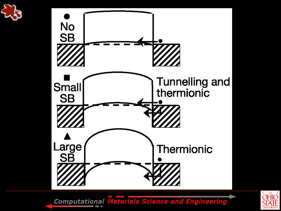
69. CNT-FET as Schottky JunctionV o
Metal lead
CNT
Lead
CNT E o
Vacuum level CB CB
CNT L EF
B = L – CNT VB EF EF VB
Before contact
After contact
Desirable: B = 0 to minimize contact resistance.
Metals with “right” B: Pt, Ti, Pd.

71. Notice the difference in the y-axis
Notice the difference in the y-axis. The X structure (below) carries a current which is about one order of magnitude smaller than the CNT inline with the contacts (left)
The main peak in the X structure is located at ~5 V, which is close to the value from the inline structure (~5.5 V). This indicates that the qualitative features in the conductance derive from the CNT while the magnitude of the conductance is set by the contacts. The extra peaks seen on the right may be due to incomplete relaxation.

72. Current (A)

73. PDOS for the relaxed CNT in line with contacts
PDOS for the relaxed CNT in line with contacts. The two curves correspond to projections on atoms far away from the two interfaces. A (3,3) CNT is metallic, still there is a gap of about 4 eV. Does the gap above result from interactions with the slabs or from lack of kpts along z? This question is not so important since the Fermi level is deep into the CNT valence band.