1. combinatorial designs
The weights of eight objects are to be measured using a pan balance and set of standard weights.
Each weighing measures the weight difference between objects placed in the left pan vs. any objects placed in the right pan by adding calibrated weights to the lighter pan until the balance is in equilibrium.
Each measurement has a random error ~ iid N(0, 2)
Denote the true weights by
How to measure them with highest accuracy with only 8 measurements?

2. Two designs D Weigh each object in one pan, with the other pan empty
Do the eight weighings according to the following schedule, let Yi be the measured difference for i = 1, ..., 8: D

3. inverse(D)=1/8* Comparison
Then the estimated value of the weight θ1 is
Similar estimates can be found for the weights of the other items. For example
Thus if we use the second experiment, the variance of the estimate given above is σ2/8.
The variance of the estimate X1 of θ1 is σ2 if we use the first experiment.

4. Full Factorial 23
Fractional Factorial 27-4

5. Chapter 4 Full Factorial Experiments at Two Levels
A 2k full factorial design
can study k factors each at two levels
has 2 × 2 × × 2 = 2k observations
can study the linear effect of the response over the range of the factor levels chosen.

6. 4.1 An Epitaxial Layer Growth Experiment
One of the initial steps in fabricating integrated circuit (IC) devices is to grow an epitaxial layer on polished silicon wafers. The wafers are mounted on a six-faceted cylinder (two wafers per facet) called a susceptor which is spun inside a metal bell jar. The jar is injected with chemical vapors through nozzles at the top of the jar and heated. The process continues until the epitaxial layer grows to a desired thickness.
4 experimental factors (labeled A, B, C and D), each at 2 levels
16 treatments, each producing 6 readings from 6 facets.
Goal: To find process conditions (i.e., combinations of factor levels for A, B, C and D) under which the average thickness is close to the (nominal) target 14.5 microns with variation as small as possible.
Analysis: focus on both average and variation of the responses.

7. The AT&T experiment based on 24 design; four factors each at two levels. There are 6 replicates for each of the 16 (=24) level combinations; data given on the next page.

10. 4.2 Full Factorial Designs at Two Levels: A General Discussion
The 2k full factorial design
2×2×. . .×2 = 2k design.
consists of all 2k combinations of the k factors taking on two levels.
has 2k treatments or runs. A treatment is a combination of factor levels.
two levels are represented by −/+, 0/1 or −1/ +1.
For quantitative factors, use − (0, −1) for the lower level and + (1, +1) for the higher level.

11. 2k Designs:
For carrying out the experiment, a planning matrix should be used to display the experimental design in terms of the actual factor levels.
The planning matrix avoids any confusion or misunderstanding of the experimental factors and levels. See Table 4.3 on page 158.
Randomization reduces the unwanted effects of other variables not in the planning matrix.
The order of the runs in the planning matrix should been randomized.
The actual run order should be different from the order of runs in the design matrix.

13. 2k Designs:
Fig. 4.1 (on page 159): An example of a lurking variable, room humidity which may increase during the day.
If the experiment is carried out over this time period and in the order given in the design matrix, the factor A (rotation method) effect would be confounded with the humidity effect.
Some factors may be hard to change, e.g., deposition temperature. Then one can do restricted randomization, i.e., randomizing the other factor levels for each level of the hard-to-change factor. See Table 4.4 on page 160.

14. Fig 4.1

16. Remark Distinction among
design matrix: (factors A,B,C,D, levels −/+, systematic order)
planning matrix: (actual factors and levels, randomized run order)
model matrix: the X matrix in linear model

17. Two key properties of the 2k designs are
balance: each factor level appears in the same number of runs.
orthogonality: all level combinations of any two factors appear in the same number of runs.
Hyper-orthogonality : all level combinations of any three+ factors appear in the same number of runs.
Fig. 4.2 and 4.3: Graphic representation of 23 and 24 designs.
The experiment can be replicated or unreplicated. Distinction between replicates and repetitions.
Q: Is the epitaxial layer growth experiment replicated or unreplicated?
Q: Are the observations from each run replicates or repetitions?

18. Fig 4.3

19. 4.3 Factorial Effects and Plots

20. 4.3.1 Main Effects Main effect of A is defined as
Another key property of the 2k designs:
reproducibility of conclusions in similar experiments.
because ¯z(A+) and ¯z(A−) are computed over all level combinations of the other factor.

21. The main effects plot graphs the averages of all the observations at each level of the factor and connects them by a line.
For two-level factors, the vertical height of the line is the difference between the two averages, which is the main effect.

22. 4.3.2 Interaction Effects
The interaction effect (A × B) between A and B can be defined as:

24. Remark.
The advantage of the first two definitions is that the interaction (which is a second order effect) is defined in terms of the difference of two conditional main effects (which are both first order effects).
Although the third definition is algebraically simpler, it is not related to the main effects of A or B and the two groupings are not easily interpretable.

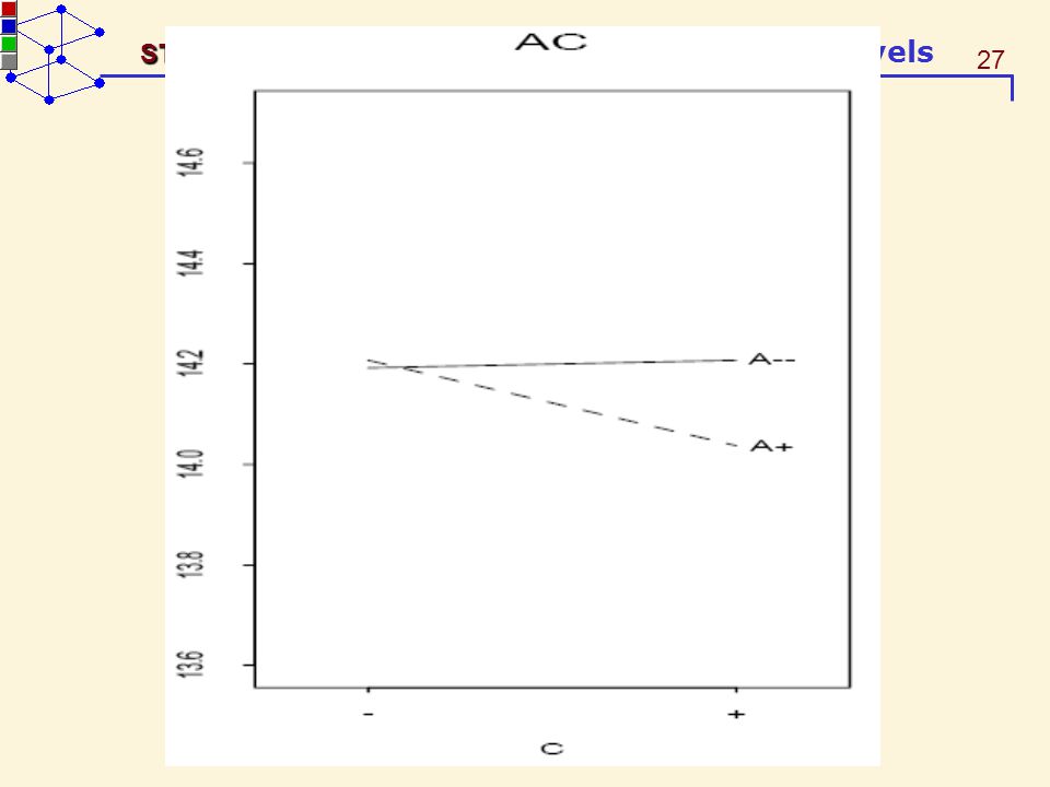
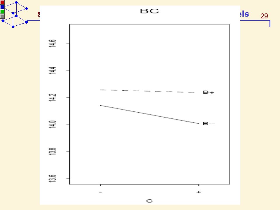
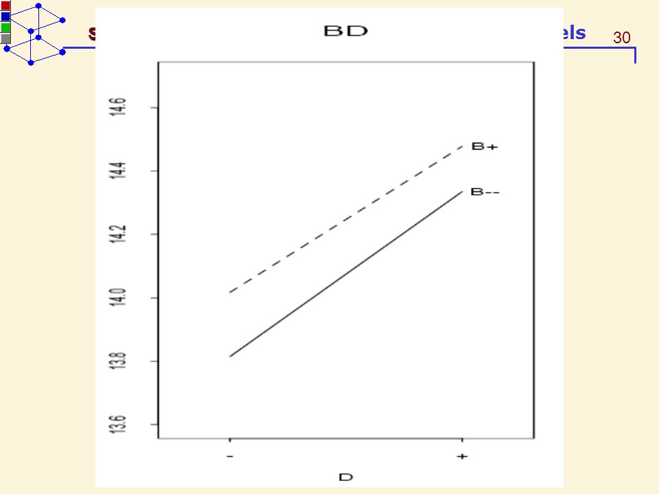
25. The interaction plots
The interaction plots display the average at each of the combinations of the two factors A and B.
The A-against-B plot use the B factor level as the horizontal axis and join the averages having the same level of A by a line.
The vertical distances of the joined lines are equal to the ME(B|A+) and ME(B|A−).

32. An A-against-B plot is called
synergystic if ME(B|A+)ME(B|A−) > 0
antagonistic if ME(B|A+)ME(B|A−) < 0.
An antagonistic plot suggests a more complex underlying relationship than what the data reveal.

33. The three-factor interaction
The three-factor interaction (A × B × C ) can be defined in terms of conditional 2-factor interactions as follows:
Or defined as the difference between two group averages

34. The A×B ×C interaction can be plotted in three different ways: (A,B)-against-C, (A,C)-against-B, and (B,C)-against-A.
For the (A,B)-against-C plot, draw a line that connects the values at the C+ and C− levels for each of the four-level combinations (−,−), (−, +), (+,−) and (+, +) of A and B.
Higher-order interactions. Define the k-factor interaction as follows:

36. Factorial effects for the adapted epitaxial layer growth experiment.
data epi;
input id A B C D y1-y6;
m=mean(of y1-y6); s=std(of y1-y6); logs=log(s**2);
AB=A*B; AC=A*C; AD=A*D; BC=B*C; BD=B*D; CD=C*D;
ABC=AB*C; ABD=AB*D; ACD=AC*D; BCD=BC*D; ABCD=ABC*D;
cards;
……………………………………… ;
proc sql;
select " A" as Factor, sum(m*(A=1))/8 as mH, sum(m*(A=-1))/8 as mL, sum(m*A)/8 as mEff, sum(logs*(A=1))/8 as sH, sum(logs*(A=-1))/8 as sL, sum(logs*A)/8 as sEff from epi union
select " B" as Factor, sum(m*(B=1))/8 as mH, sum(m*(B=-1))/8 as mL, sum(m*B)/8 as mEff, sum(logs*(B=1))/8 as sH, sum(logs*(B=-1))/8 as sL, sum(logs*B)/8 as sEff from epi union

37. SAS output

38. 4.4 Using Regression Analysis to Compute Factorial Effects
Consider the 23 design for factors A, B and C, whose columns are denoted by x1, x2 and x3 (=1 or -1).
The interactions AB, AC, BC, ABC are then equal to
x4 = x1x2,x5 = x1x3,x6 = x2x3,x7 = x1x2x3
Use the regression model
where i = ith observation.
The regression (i.e., least squares) estimate of bj is

39. Model Matrix for 23 Design
AB = A*B,
AC = A*C,
BC = B*C,
ABC = A*B*C

40. Factorial Effects, Adapted Epi-Layer Growth Experiment
The linear model for the epitaxial layer growth experiment is
If we code levels +/− as +1/−1, the least squares estimates are half the factorial effects.
Therefore, each factorial effect can be obtained by doubling the corresponding regression estimate.

41. proc reg outest=effects data=epi1; /. REG Proc to Obtain Effects
proc reg outest=effects data=epi1; /* REG Proc to Obtain Effects */ model m=A B C D AB AC AD BC BD CD ABC ABD ACD BCD ABCD; run;

42. 4.6 Fundamental Principles for Factorial Effects
Three fundamental principles are often used to justify the development of factorial design theory and data analysis strategies.
Hierarchical Ordering Principle:
(i) Lower order effects are more likely to be important than higher order effects.
(ii) Effects of the same order are equally likely to be important.
This principle suggests that when resources are scarce, priority should be given to the estimation of lower order effects.
It is an empirical principle whose validity has been confirmed in many real experiments.
Another reason for its wide acceptance is that higher order interactions are more difficult to interpret or justify physically.

43. Fundamental Principles for Factorial Effects
Effect Sparsity Principle: The number of relatively important effects in a factorial experiment is small.
The principle may also be called the Pareto Principle in Experimental Design because of its focus on the “vital few” and not the “trivial many.”
Effect Heredity Principle: In order for an interaction to be significant, at least one of its parent factors should be significant.
This principle governs the relationship between an interaction and its parent factors and can be used to weed out incompatible models in searching for a good model.

44. 4.7 One-Factor-At-A-Time (ofat) Approach
The one-factor-at-a-time approach (commonly used in scientific and engineering investigations):
(i) identify the most important factor,
(ii) investigate this factor by itself, ignoring the other factors,
(iii) make recommendations on changes (or no change) to this factor,
(iv) move onto the next most important factor and repeat steps (ii) and (iii).

45. One-Factor-At-A-Time (ofat) Approach
Disadvantages of the one-factor-at-a-time approach:
1. It requires more runs for the same precision in effect estimation.
2. It cannot estimate some interactions.
3. The conclusions from its analysis are not general.
4. It can miss optimal settings of factors.

46. Example: Comparison of two-factor designs.

47. (ofat) Example: an injection molding process
goal: to reduce the percentage of burned parts.
3 factors are injection pressure (P: psi), screw rpm control (R: turns counterclockwise) and injection speed (S: slow-fast).
The design matrix and response of a 23 factorial design.

48. ofat
Step 1. Factor P is thought to be the most important. Fix the other factors at standard conditions (R=0.6, S=fast) and compare 2 levels of P. Choose P=1200.
Step 2. The next most important factor is thought to be R. Fix P=1200 and S=fast (standard condition), compare 2 levels of R. Choose R=0.3.
Step 3. Fix P=1200 and R=0.3 and compare 2 levels of S. Choose S=slow.
The final percentage burn at P=1200, R=0.3 and S=slow is 11.
A possible Path of
One-Factor-At-A-Time Plan

49. Factorial Effects from the 23 factorial design

51. In the example, the 23 design requires 8 runs
In the example, the 23 design requires 8 runs. For ofat to have the same precision, each of the 4 corners on the ofat path needs to have 4 runs, totaling 16 runs.
In general, to be comparable to a 2k design, ofat would require 2k−1 runs at each of the k+1 corners on its path, totaling (k+1)2k−1.
The ratio is (k+1)2k−1/2k = (k+1)/2.

52. Var(MEA)=1/4*(σ2+σ2) +1/4*(σ2+σ2)=σ2 ME(A)=y1-y3 Var(MEA)=σ2+σ2=2σ2
ME(A)=1/2(y1+y2) /2(y3+y3)
Var(MEA)=1/4*(σ2+σ2)
+1/4*(σ2+σ2)=σ2
ME(A)=1/2(y11+y12) /2(y31+y32)
Var(MEA)=1/4*(σ2+σ2) /4*(σ2+σ2)=σ2
ME(A)=y1-y3
Var(MEA)=σ2+σ2=2σ2
The 22 design requires 4 runs, For ofat to have the same precision, each of the 3 corners on the ofat path needs to have 2 runs, totaling 6 runs;
The 23 design requires 8 runs. For ofat to have the same precision, each of the 4 corners on the ofat path needs to have 4 runs, totaling 16 runs.
In general, to be comparable to a 2k design, ofat would require 2k−1 runs at each of the k+1 corners on its path, totaling (k+1)2k−1.
The ratio is (k+1)2k−1/2k = (k+1)/2.

53. Why Experimenters Continue to Use ofat?
Most physical laws are taught by varying one factor at a time. Easier to think and focus on one factor each time.
Experimenters often have good intuition about the problem when thinking in this mode.
No exposure to statistical design of experiments.
Challenges for DOE researchers: To combine the factorial approach with the good intuition rendered by the the ofat approach. Needs a new outlook.

54. 4.8 Effect of Simultaneous Testing
Main idea: comparing all factorial effects simultaneously is like doing multiple comparisons.

55. 4.8 Normal and Half-Normal Plots
Normal and half-normal plots are useful graphical tools to judge effect significance.
are informal but effective method
do not require to be estimated.
do not suffer from the effect of simultaneous testing.

56. the normal probability plot of location effects from the adapted epitaxial layer growth experiment. It suggests that only D, CD (and possibly B) are significant.

57. 4.8 Use of Normal Plot to Detect Effect Significance
Deduction Step. Null hypothesis H0: all factorial effects=0. Under H0, and the resulting normal plot should follow a straight line.
Induction Step. By fitting a straight line to the middle group of points (around 0) in the normal plot, any effect whose corresponding point falls off the line is declared significant (Daniel, 1959).
Unlike t or F test, no estimate of s2 is required. Method is especially suitable for unreplicated experiments. In t test, s2 is the reference quantity. For unreplicated experiments, Daniel’s idea is to use the normal curve as the reference distribution.
In previous Figure, D, CD (and possibly B?) are significant. Method is informal and judgemental.

58. Normal plot can be misleading.
Half-normal plots are preferred for testing effect significance.

60. Visual Misjudgement with Normal Plot
Potential misuse of normal plot :
In previous Figure (top), by following the procedure for detecting effect significance, one may declare C, K and I are significant, because they “deviate” from the middle straight line.
This is wrong because it ignores the obvious fact that K and I are smaller than G and O in magnitude.
This points to a potential visual misjudgement and misuse with the normal plot.

61. 4.9 A Formal Test of Effect Significance : Lenth’s Method

62. A Formal Test of Effect Significance (Contd.)

63. Two Versions of Lenth’s Method

64. Illustration with Adapted Epi-Layer Growth Experiment

65. Table 4.9: |tPSE| Values, Adapted Epitaxial Layer Growth Experiment
Effect y lns2 BC BD CD
ABC
ABD
ACD
BCD
ABCD
Effect y lns2 A B C D AB AC AD

66. 4.10 Nominal-the-Best Problem and Quadratic Loss Function
Nominal-the-best problem: to keep the thickness deviation from the nominal or target t = 14.5 microns as small as possible.
Quadratic loss function: loss of the deviation of the response y from target t
where c is a constant determined by other considerations such as cost or financial loss. Note
Therefore, the expected loss can be minimized or reduced by selecting some factor levels (i) that minimize the variance Var(y) and (ii) that move the mean E(y) closer to the target t.

67. Two-Step Procedure for Nominal-the-Best Problem
(i) Select levels of some factors to minimize Var(y),
(ii) Select the level of a factor not in (i) to move E(y) closer to t.
A factor in Step (ii) is called an adjustment factor if it has a significant effect on the mean E(y) but not on the variance Var(y).
Procedure is effective only if an adjustment factor can be found. This is often done on engineering ground.
(Examples of adjustment factors : deposition time in surface film deposition process, mold size in tile fabrication, location and spacing of markings on the dial of a weighing scale).
Without the existence of an adjustment factor, the two-step procedure would not be effective. Then it is desirable to minimize the loss function L(y, t) directly.

68. 4.11 Log Transformation of the Sample Variances - Why Take ln s2 ?
It maps s2 over (0,) to ln s2 over (−,). Regression and ANOVA assume the responses are nearly normal, i.e. over (−,).
Better for variance prediction. Suppose z = lns = predicted value of lns2, then = predicted variance of s2, always nonnegative.
Most physical laws have a multiplicative component. Log converts multiplicity into additivity.
Variance stabilizing property.

69. 4.12 Analysis of Location and Dispersion Epi-layer Growth Experiment Revisited

70. Epi-layer Growth Experiment: Effect Estimates
By regression

71. Epi-layer Growth Experiment: Half-Normal Plots

73. 4.15 Blocking and Optimal Arrangement of 2k Factorial Designs in 2q blocks
Blocking is necessary when it is impossible to perform all of the runs in a 2k factorial experiment under homogeneous conditions.

74. Blocking a replicated 2k factorial design
Example: The investigation of the effect of (A) the concentration of reactant and (B) the amount of the catalyst on the conversion (yield) in a chemical process.
Only 4 experimental trials can be made from a single batch of raw material.
Three batches of raw material are used to run all 3 replicates.
This is a complete block design (Each batch forms a block; all 4 treatments are compared in each block).

75. model y=A B AB Batch/solution; run;
data d;
input A B Batch y;
AB=A*B;
cards; ;
proc GLM;
class Batch;
model y=A B AB Batch/solution;
run;

76. Blocking a replicated 2k factorial design
Linear model is
Here the block effect is not significant. Both main effects A and B are significant, but their interaction is not.

77. Standard
Parameter Estimate Error t Value Pr > |t|
Intercept B <.0001 A B AB
Batch B
Batch B
Batch B

78. Estimates under baseline constraints (for block effects) are

79. proc GLM; class Batch; model y=A B AB Batch/solution; run;
data d;
input A B Batch y;
AB=A*B;
cards; ;
Standard
Parameter Estimate Error t Value Pr > |t|
Intercept B <.0001 A B AB
Batch B
Batch B
Batch B

80. Blocking a unreplicated 2k factorial design
When k is moderately large, a 2k factorial design is often unreplicated and therefore it is impossible to have a complete block design.
Then an incomplete block design can be used.
The price to pay is that some factorial effects will be confounded with block effects and cannot be estimated.

81. Example: To arrange a 22 design in 2 blocks:
-++-
Example: To arrange a 22 design in 2 blocks:
The factorial effects are
But we have a block variable. The block effect is
The block effect and INT(A,B) have the same estimate.
The 2-factor interaction AB is confounded with the block effect.

82. If blocking is effective, the block effect should be large.
Cannot estimate AB.
Both main effects A and B are not affected by the block effect (WHY?).
Randomized block design?

83. Example: To arrange a 23 design in 2 blocks:
23 design can estimate 7 factorial effects: 1, 2, 3, 12, 13, 23, 123.
When it is arranged in 2 blocks, we have to sacrifice one factorial effect.
Based on the hierarchical ordering principle (Section 3.5), the three-factor interaction is the least important and should be sacrificed.
The blocking scheme:
Block I if the entry in the 123 column is −,
Block II if the entry in the 123 column is +,

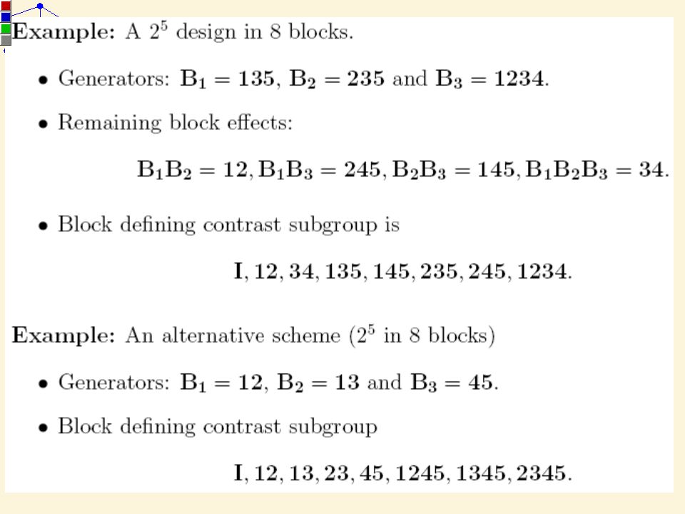
85. Example: To arrange a 23 in 4 blocks.
Define two blocking variables B1 = 12 and B2 = 13, which divides the 8 runs into 4 blocks according to

86. Example: To arrange a 23 in 4 blocks.
There are 3 block effects among 4 blocks; therefore, 3 factorial effects are confounded with the block effects.
The third block effect B3 = B1B2 is confounded with 23 interaction, because
where I is the column of +’s.

87. An alternative blocking scheme:
However, the third block effect is
a very bad scheme: the main effect 2 is confounded with a block effect.
Assumption:
The block-by-treatment interactions are negligible.
That is, the treatment effects do not vary from block to block. The validity of the assumption has been confirmed in many empirical studies.
It can be checked by plotting the residuals for all the treatments within each block. If the pattern varies from block to block, the assumption may be violated.

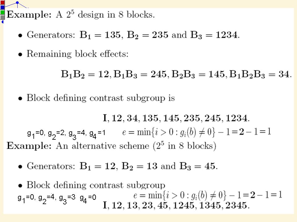
88. Arrange a 2k design in 2q blocks of size 2k−q

91. (No main effect should be confounded with block effects)