Download presentation
Presentation is loading. Please wait.

1
Mark Ortel Sales Support Eng
Sweep Overview Mark Ortel Sales Support Eng

2
Conditioning the Network for Triple Play Services
Know Your HFC Network System Sweep and Ingress Suppression Testing and Hardening the Drop (Home Wiring) Line Conditioning to Optimize Two-way Plant Performance Fiber Optic Testing Maintenance In the days before the introduction of hybrid fiber/coaxial ‘HFC’ networks, plant design and alignment were considerably simpler: there was one dominant architecture (‘trunk and branch’) and a restricted set of amplifier operating levels. Furthermore, the reverse path was designed almost as an ‘afterthought’. Since the only reverse signals were likely to be one or two analog video channels and a Status Monitoring signal, a less than optimal design, and an ‘as-required’ activation and alignment procedure were usually adequate.
 Line Conditioning to Optimize Two-way Plant Performance. Fiber Optic Testing Maintenance. In the days before the introduction of hybrid fiber/coaxial ‘HFC’ networks, plant design and alignment were considerably simpler: there was one dominant architecture (‘trunk and branch’) and a restricted set of amplifier operating levels. Furthermore, the reverse path was designed almost as an ‘afterthought’. Since the only reverse signals were likely to be one or two analog video channels and a Status Monitoring signal, a less than optimal design, and an ‘as-required’ activation and alignment procedure were usually adequate.")
3
Bandwidth Demand is Growing Exponentially
All Video on Demand Unicast per Subscriber 100 90 High Definition Video on Demand 80 Video Blogs 70 Podcasting 60 Megabits per Second Video on Demand 50 Video Mail 40 Online Gaming 30 Digital Photos 20 VoIP Digital Music 10 Web Browsing Time

4
Home Is Where The Net Is Cable is THE BROADBAND of choice
Intelligent network Mix of IP and MPEG Multiple businesses & services, one network Best in Class Security, provisioning, management Voice, data, video convergence For the service provider, a converged network means Common provisioning/management/security For the consumer, a converged application means Device-independence Same “look and feel” Ease of use, plug and play

6
Voice Quality Impairments – it’s not always the plant!
Telco Problem? Customer Problem? Cable Provider Problem? Cable Provider Problem? Where is the Problem? What is the Problem? PSTN analog problems on PSTN path passed through to IP network MEDIA GW POP DSP codec performance, echo canceller config., jitter buffer config. / packet drops CORE IP NTWK High utilization lead to congestion causing jitter, dropped packets and increased transit delay, mis-configured routing can cause inappropriate hops leading to increased latency HUB SITE Excessive NE polling and/or high utilization lead to congestion causing jitter, dropped packets and increased transit delay HUB SITE CABLE PLANT RF downstream and/or upstream errors leading to IP packet loss, bandwidth capacity limitations (esp. upstream) may lead to CMTS congestion (dropped IP packets) and excessive jitter (packet drops by codec) HOME Background noise, handset speaker/mic interference, inadequate volume, inside wiring, mis-configured MTA (CoS-Diffserv / firewall settings), wireless phone delay exacerbates echo problems, MTA DSP/echo canceller performance Router-Slot-Port? LSP/VLAN, Route? What’s the problem? MEDIA POP Aggregation switch CMTS MediaGW-Slot-Port? DSP Card-Port-CPU? What’s the problem? Cable PSTN Trunk Media Gateway CMTS Core IP Network CMTS CMTS-Blade-Port or Switch-Slot-Port? What’s the problem? UPSTREAM or DOWNSTREAM? What’s the problem? MEDIA POP Cable Modem MTA POTS Phone Trunk Media Gateway
 may lead to. CMTS congestion (dropped. IP packets) and excessive. jitter (packet drops by codec) HOME. Background noise, handset. speaker/mic interference, inadequate volume, inside. wiring, mis-configured MTA. (CoS-Diffserv / firewall. settings), wireless phone. delay exacerbates echo. problems, MTA DSP/echo. canceller performance. Router-Slot-Port LSP/VLAN, Route What’s the problem MEDIA POP. Aggregation. switch. CMTS. MediaGW-Slot-Port DSP Card-Port-CPU What’s the problem Cable. PSTN. Trunk Media. Gateway. CMTS. Core IP. Network. CMTS. CMTS-Blade-Port or Switch-Slot-Port What’s the problem UPSTREAM or. DOWNSTREAM What’s the problem MEDIA POP. Cable. Modem. MTA. POTS. Phone. Trunk Media. Gateway.")
7
‘Pre-HFC’ Networks No Optics Standardized ‘Tree & Branch’ Architecture
Few Amplifier Types Limited Operating Levels Networks were optimized for forward plant performance with minimal reverse plant engineering. In the days before the introduction of hybrid fiber/coaxial ‘HFC’ networks, plant design and alignment were considerably simpler: there was one dominant architecture (‘trunk and branch’) and a restricted set of amplifier operating levels. Furthermore, the reverse path was designed almost as an ‘afterthought’. Since the only reverse signals were likely to be one or two analog video channels and a Status Monitoring signal, a less than optimal design, and an ‘as-required’ activation and alignment procedure were usually adequate.
 and a restricted set of amplifier operating levels. Furthermore, the reverse path was designed almost as an ‘afterthought’. Since the only reverse signals were likely to be one or two analog video channels and a Status Monitoring signal, a less than optimal design, and an ‘as-required’ activation and alignment procedure were usually adequate.")
8
‘Pre-HFC’ Networks No Optics Standardized ‘Tree & Branch’ Architecture
Few Amplifier Types Limited Operating Levels Networks were optimized for forward plant performance with minimal reverse plant engineering. Headend In the days before the introduction of hybrid fiber/coaxial ‘HFC’ networks, plant design and alignment were considerably simpler: there was one dominant architecture (‘trunk and branch’) and a restricted set of amplifier operating levels. Furthermore, the reverse path was designed almost as an ‘afterthought’. Since the only reverse signals were likely to be one or two analog video channels and a Status Monitoring signal, a less than optimal design, and an ‘as-required’ activation and alignment procedure were usually adequate.
 and a restricted set of amplifier operating levels. Furthermore, the reverse path was designed almost as an ‘afterthought’. Since the only reverse signals were likely to be one or two analog video channels and a Status Monitoring signal, a less than optimal design, and an ‘as-required’ activation and alignment procedure were usually adequate.")
9
HFC Networks Combines fiber optics with coaxial distribution network
Return path is more sensitive than the forward path Most of the ingress comes from home wiring on low value taps Wide variety of hardware with many connectors Today’s ‘HFC” networks must be optimized for both forward and reverse performance The introduction of fiber optics to the broadband industry and the proliferation of different architectures (originated by both vendors and operators) has added complexity to the issues of reverse path design and implementation. Also, the number of actual and potential interactive services is increasing, with a wide range of data rates and modulation schemes. These signals have different transmission requirements in terms of carrier-to-noise ratio and received signal level. Since the ‘forward’ plant design differs from system to system, there are no universal rules which allow reverse operating parameters to be set by a simple formula.
 has added complexity to the issues of reverse path design and implementation. Also, the number of actual and potential interactive services is increasing, with a wide range of data rates and modulation schemes. These signals have different transmission requirements in terms of carrier-to-noise ratio and received signal level. Since the ‘forward’ plant design differs from system to system, there are no universal rules which allow reverse operating parameters to be set by a simple formula.")
10
HFC Network Architecture
NODE

11
HFC Network Architecture
NODE

12
Upstream Optical Receivers
Basic DOCSIS® Network Downstream Laser and Upstream Optical Receivers CMTS Fiber Nodes Cable Modems Downstream 0 Upstream 0 Cable Modems Upstream 1 Cable Modems Upstream 2 Cable Modems Upstream 3 Coax Fiber Coax

13
Types of Lasers used in HFC Networks
Fabry-Pérot (FP) Less Expensive Mediocre Performance No Isolation or Cooling Required Distributed Feedback (DFB) Expensive High Performance Isolation and Cooling Required
 Less Expensive. Mediocre Performance. No Isolation or Cooling Required. Distributed Feedback (DFB) Expensive. High Performance. Isolation and Cooling Required.")
14
Constant Outputs with Variable Inputs Fixed Signals System Noise
Forward System Diverging System Constant Outputs with Variable Inputs Fixed Signals video / audio / digital carriers System Noise is the sum of cascaded amplifiers Balance or Align (Sweep) compensate for losses before the amp 6 6
 compensate for losses before the amp")
15
Forward Path Unity Gain
OUT +36 dBmV IN +12 dBmV OUT +36 dBmV IN +11 dBmV OUT +36 dBmV 2 dB MHz 8 dB MHz AMP # 1 AMP # 2 AMP # 3 MHz IN +10 dBmV AMP # 4 OUT +36 dBmV

16
Constant Inputs with Variable Outputs No Fixed Signals System Noise
Reverse System Converging System Constant Inputs with Variable Outputs No Fixed Signals impulse digital carriers System Noise is the sum of all active components Balance or Align (Sweep) compensate for losses after the amp 7 7
 compensate for losses after the amp")
17
Return Path Unity Gain IN +20 dBmV OUT +24 dBmV IN +20 dBmV OUT
4 40 MHz 8 dB 4 40 MHz AMP # 1 AMP # 2 AMP # 3 2 40 MHz OUT +30 dBmV AMP # 4 IN +20 dBmV

18
Reverse Path Impairments
Ingress and electrical noise Common Path Distortion (CPD) Thermal (intrinsic) noise Laser clipping noise Micro-Reflections The key concern in the reverse path is noise, either from outside sources (ingress) or intrinsic to the system. The intrinsic noise sources include: RF amplifier thermal noise Optical link noise - laser clipping noise - Relative Intensity Noise (RIN) - Mode Dispersion Noise (MDN) - Rayleigh scattering (due to molecular imperfections in the optical fiber glass) It is usually possible to combine the RF amplifier noise, RIN and MDN into a single ‘noise floor’ figure. Laser clipping noise, on the other hand, should be calculated on the basis of the known and projected reverse traffic, and the characteristics of the reverse laser.
 Thermal (intrinsic) noise. Laser clipping noise. Micro-Reflections. The key concern in the reverse path is noise, either from outside sources (ingress) or intrinsic to the system. The intrinsic noise sources include: RF amplifier thermal noise. Optical link noise. - laser clipping noise. - Relative Intensity Noise (RIN) - Mode Dispersion Noise (MDN) - Rayleigh scattering (due to molecular imperfections in the optical fiber glass) It is usually possible to combine the RF amplifier noise, RIN and MDN into a single ‘noise floor’ figure. Laser clipping noise, on the other hand, should be calculated on the basis of the known and projected reverse traffic, and the characteristics of the reverse laser.")
19
Reverse Path Impairments
There are a variety of impairments that can affect two-way operation. They are classified in three main categories: stationary impairments, which include thermal noise, intermodulation distortion,and frequency response problems; transient impairments, which include RF ingress, impulse noise, and signal clipping; and multiplicative impairments, which include transient hum modulation and intermittent connections.

20
Reverse Path Impairments
Thermal noise —The majority of thermal noise is generated in active components. Besides choosing active equipment with a relatively low noise figure, there is little else that you can do about the thermal noise in active devices, other than ensure proper network alignment.

21
Reverse Path Impairments
Intermodulation distortion—The most common types of intermodulation distortion affecting the reverse path are second and third order distortions. These can be generated in amplifiers and reverse lasers. A more troubling type of intermodulation can occur in some passive components. It is known as common path distortion (CPD), and usually occurs at a dissimilar metals interface where a thin oxide layer has formed.
, and usually occurs at a dissimilar metals interface where a thin oxide layer has formed.")
22
Reverse Path Impairments
Frequency response— Frequency response problems are due to improper network alignment, unterminated lines, or damaged components. When reverse frequency response and equipment alignment have been done incorrectly or not at all, the result can be excessive thermal noise, distortions, and group delay errors.

23
Reverse Path Impairments
RF ingress — The 5-40 MHz reverse spectrum is shared with numerous over-the-air users. Signals in the over-the-air environment include high power shortwave broadcasts, amateur radio, citizens band, government, and other two-way radio communications.

24
Downstream and Upstream Noise Additions
Headend Headend Ingress from seven amplifiers ends up at the headend. Reverse System “Noise Funneling” Forward Signals Noise Noise

25
Reverse Path Impairments
Impulse noise —Most reverse data transmission errors have been found to be caused by bursts of impulse noise. Impulse noise is characterized by its fast risetime and short duration. Common sources include vehicle ignitions, neon signs, static from lightning, power line switching transients, electric motors, electronic switches, and household appliances.

26
Impulse Noise in the Upstream

27
Sample: “Loose Plant” Performance History
Average noise floor at 17 MHz varies consistently by time of day Indication of return path with an ingress problem. Maintenance now will prevent future problems 11:00PM 7:00AM 11:00PM 7:00AM Single Frequency Time Window for 72 Hours from one return path

28
Sample: ‘Tight’ Performance History
17 MHz noise floor tracked over time Average noise floor stays fairly flat and consistent over the 3 day period Inconsistent Problem (high peak, low average) Peak Average Minimum Single Frequency Time Window for 72 Hours from one return path
 Peak. Average. Minimum. Single Frequency Time Window for 72 Hours from one return path.")
29
Sample: “Telephony” Performance History
Average telephony signal at 36 MHz varies consistently by time of day Indication of higher telephony usage times 11:00PM 7:00AM 11:00PM 7:00AM Single Frequency Time Window for 3 days from one return path

30
6MHz CPD

31
Reverse Path Impairments
Signal clipping —RF ingress and impulse noise can cause signal clipping, or compression, in reverse plant active components. Excessive levels from in-home devices such as pay-per-view converters also can cause clipping. Clipping occurs in reverse amplifiers and optical equipment.

32
Ingress 75 – 90% of ingress originates in the subscriber’s home
To minimize the effects of ingress, operate the subscriber terminals (modems & set-tops) near maximum transmit level A key objective of the reverse design strategy should be to arrange for all subscriber terminals to operate at or near their maximum RF output level. This will help significantly to overcome the effects of ingress. Also, in the case of devices with user-adjustable output levels, it will prevent accidental or deliberate increase in reverse level (a ‘hot talker’). Tracking Down Ingress The first step is to verify it is truly on your network and not self-induced. Use some type of spectrum analyzer to view the anomaly. Cross reference with frequency charts that identify different ingress sources to get a best-guess idea. Noise and transient ingress above the diplex filter region is probably laser clipping or induced at the node. You may also want to view the frequencies below 5 MHz to verify it’s clean. Noise below 5 MHz could still affect the laser’s dynamic range. Listening to Ingress for Identification of the Source The second step is to demodulate the ingress, if possible, to identify the type of ingress. Reverse path ingress is usually amplitude modulated (AM), but could also be FM. Listening to the ingress helps to identify the source. • FM demod for the audio of forward channels and certain shortwave radio. • AM demod for most reverse interference and ingress, such as CB, Ham, and shortwave radio. • This may give you some insight into the location of the source or at least the nature of the source. You may be able to get the call signs of a ham radio operator or a mile marker from a truck driver using his CB. This could aid in pinpointing the ingress location. A single source of interference is easy to track down. If it’s constant, just use the "divide and conquer" theory to dissect the system. Observing how it reacts and changes could indicate different sources such as a trucker or home user. A CB level changing quickly or slowly could indicate this source quickly. Multiple ingress sources, bursty noise, and electrical transient noise are a totally different story and are very difficult to pinpoint. Remember that the lower value taps contribute more noise and ingress than the higher value taps. The lower attenuation from tap values of 14 and below coupled with the low attenuation in the cable at lower frequencies creates an easy path for noise to funnel back. Test Location Considerations • Because the return path signals are low in level, it may be warranted to use a preamp. • The preamp is used to raise the signal above the noise floor of the test equipment. This is especially a problem on the return signals that are read from high loss test points. • The newer units have a preamp built-in and compensate all measurements accordingly. • If a problem is observed at the output seizure screw of a tap, continue on. • Some new probes from SignalVision and Gilbert create a good ground and quick connect. Note: One caveat to this is a probe will always be bi-directional and will cause an impedance mismatch itself. This is something to keep in mind when troubleshooting. Sometimes an in-line pad can be attached to decrease the amount of energy tested, which in turn, may create a better match. Be careful when probing seizure screws, though. The AC present will harm in-line pads and certain test equipment. The equipment is AC blocked for ~ 100 Vac. • Start with 14 dB taps and lower. If the problem is at the input of the tap and not the output, then the problem is from one of the drops or farther upstream possibly from a cracked cable before the next amplifier. • Look at one drop at a time to determine the biggest contributor. Noise Readings • Be careful with spectrum analyzer, noise level readings. 2 dB/div is a good scale for sweeping and 5 or 10 dB/div is best for the spectrum mode. • The level displayed is based on the RBW setting and will be very different from one setting to another. A -20 dBmV noise floor with 30 kHz RBW is really 1.2 dBmV in a 4 MHz bandwidth and there’s usually a correction factor associated with it. Note: The "Spectrum" mode is not the same as a true spectrum analyzer. The RBW is set at 280 kHz and a VBW > 1 MHz. This is optimized for analog carriers and burst noise measurements. It has a peak noise detector so the noise reading may be significantly higher than a normal spectrum analyzer with the same RBW setting. • A pad on the analyzer will lower the level as well. Attenuation and gain affect noise and carriers equally. • Measurements with no point of reference are very misleading. If there’s a reference carrier present, you can make a relative measurement, such as desired-to-undesired ratio (D/U). One fault with this, though, is RBW settings affect noise and continuous wave (CW) carriers differently. A CW carrier is theoretically 1 Hz wide and the level won’t change with different RBW settings while the noise level will, thus giving a different D/U ratio. A CW carrier will change shape on the analyzer display because of the RBW filter width. The "Noise" Mode • The ability to switch between a headend mode and a remote analyzer mode has many advantages. One can successfully use the "divide and conquer" technique to quickly find the source of the problem and not have to rely on another person’s interpretation. This also eliminates inefficient use of resources and employee time. • The field unit has a "noise/ingress" feature, which can be used for troubleshooting. This displays the noise seen in the headend with optimum resolution of 280 kHz. This simplifies reverse troubleshooting and testing of headend reverse noise or ingress. The newer headend unit will transmit or broadcast the ingress from all the return amplifiers connected to it back to the field unit. This transmits the ingress seen in the headend on the forward telemetry frequency. So if no reverse communication is achieved, you will still get a display of the noise/ingress floor. The noise mode on the multiple user reverse receiver (Rx) transmits the total noise in the headend also, but with a resolution based on the return channel plan resolution. Note: The newer "Noise" mode can take up to a minute to track if the reverse is not connected. The new PathTrak system is faster and more resolution is obtained for return path monitoring and troubleshooting. PathTrak PathTrak is a Return Path Monitoring system that consistently and automatically provides: • Advanced notice to detect developing problems • A chance to respond before outages occur, which eventually generate into service calls • Performance archiving • Ability to organize preventative maintenance • Reports to correlate RF plant performance to error reports from modems and telephony systems Systems can quickly characterize and separate real problems from insignificant events. This is critical to: • Perform trend analysis • Set baseline performance standards • Certify plant as "ready" for operation • Document times and frequencies that are more reliable, possibly to set times for IPPV downloads and to do quality of service (QoS) provisioning. This system can also be incorporated to communicate with the field units. This allows the field unit to observe noise and ingress levels in the headend while in the field on a "per node" basis. Return Path Egress/Ingress Testing • The FCC states that the maximum allowable limit for egress from dc up to 54 MHz is 15 μV/m at 30 meters. We commonly refer to this as leakage. • By utilizing forward path egress techniques, it may be possible to characterize the return path ingress points to some extent. Testing stringently at 5 or 10 uV/m everywhere, including the drops, is probably a better indication of return path integrity. The hardline plant only contributes about 5% of the total ingress. Approximately 75% of ingress is from house and 20% from the drop. • Forward path leakage does not necessarily equal ingress, though. Some sources of leakage and ingress are frequency selective. This would lead us to believe that a reverse frequency would be better to monitor. • The problem with this is signals on the return path are only present when communication is taking place. They are usually very low in level and bursty in nature. • We can’t insert a reverse frequency carrier at the headend because the diplex filters would block the carrier. • We can’t insert a carrier at the EOL and look for egress, because sources of ingress inhibit accurate measurements. Most importantly, the antenna would be huge; approximately 23.4 feet for 20 MHz! Maybe we can get away with an octave of that and also tag it with an identifying signal. Using a Variable Dwell Time to Catch Impulse Noise • Some spectrum analyzers call this sweep speed or the dwell time. If the sweep speed is too fast, it may skip over fast impulse noise. • So we slow down the sweep speed or increase the dwell time. One problem with a longer dwell time on a spectrum analyzer is that it takes longer to scan. • The nice thing about a longer dwell time is that it’s easier to catch intermittent signals because it displays the carrier peak. This is similar to a peak hold every scan, which makes it great for troubleshooting impulse noise. The "Zero Span" Mode • In this mode, you can view desired-to-undesired ratios and see peak bursts of TDMA data. You can also measure peak digital levels, observe high traffic periods & collisions, and see ingress in the data packet without taking the service off-line. • Measuring the Signal-to-Noise (S/N) on return-path cable modem signals has never been an easy assignment, especially for the novice field technician. A fundamental difficulty has been the detailed set-up of the test equipment required to make the modem S/N measurement. The test equipment is normally a spectrum analyzer used in a zero-span operating mode. The zero-span mode requires the user to be well acquainted with set-up parameters such as trigger level threshold, sweep time, measurement bandwidth, video bandwidth, and resolution bandwidth. The field technician must also be proficient at RF signal evaluation in the time-domain mode, versus the standard frequency domain mode. • To overcome the confusing test equipment set-up process, Acterna has introduced a new instrument feature that allows technicians, at all skill levels, to perform accurate return-path cable modem S/N measurements. The feature is called Modem C/N, and is a standard feature on all SDA-5000 and SDA-4040D meters with firmware version 2.2. This feature is accessable under the Navigator screen. Why Measure Cable Modem C/N? • The modem S/N of the return cable plant may well determine whether the return network is capable of reliably carrying cable modem traffic. The DOCSIS standard states that the S/N for upstream (return) digital signals is 20 dB for QPSK and 25 dB for 16-QAM. Although most QPSK and 16-QAM signals are robust enough to transmit through noisier return path environments, complying with the DOCSIS S/N standard will ensure that the cable modem will reliably operate on the return network. • Use the pre-amp and low pass filter when doing any zero-span or modem test. The forward levels hitting the meter and the test equipment noise floor could give faulty noise floor readings. • The RBW is factory set to 2 MHz. To make accurate measurements in zero-span, you should use a RBW smaller than the actual payload of the modem. Remember there are 5 modem payloads specified. .16, .32, .64, 1.28, and 2.56 MHz. I'm talking payload not the filter skirts included. • You can use the factory default RBW of 2 MHz if you make the MBW 2 MHz like the RBW, that way no correction factor is added for carriers that are narrower than 2 MHz. One problem with this is the noise floor will be uncorrected when it actually should be.
 near maximum transmit level. A key objective of the reverse design strategy should be to arrange for all subscriber terminals to operate at or near their maximum RF output level. This will help significantly to overcome the effects of ingress. Also, in the case of devices with user-adjustable output levels, it will prevent accidental or deliberate increase in reverse level (a ‘hot talker’). Tracking Down Ingress. The first step is to verify it is truly on your network and not self-induced. Use some type of spectrum analyzer to view the anomaly. Cross reference with frequency charts that identify different ingress sources to get a best-guess idea. Noise and transient ingress above the diplex filter region is probably laser clipping or induced at the node. You may also want to view the frequencies below 5 MHz to verify it’s clean. Noise below 5 MHz could still affect the laser’s dynamic range. Listening to Ingress for Identification of. the Source. The second step is to demodulate the ingress, if possible, to identify the type of ingress. Reverse path ingress is usually amplitude modulated (AM), but could also be FM. Listening to the ingress helps to identify the source. • FM demod for the audio of forward channels and certain shortwave radio. • AM demod for most reverse interference and ingress, such as CB, Ham, and shortwave radio. • This may give you some insight into the location of the source or at least the nature of the source. You may be able to get the call signs of a ham radio operator or a mile marker from a truck driver using his CB. This could aid in pinpointing the ingress location. A single source of interference is easy to track down. If it’s constant, just use the divide and conquer theory to dissect the system. Observing how it reacts and changes could indicate different sources such as a trucker or home user. A CB level changing quickly or slowly could indicate this source quickly. Multiple ingress sources, bursty noise, and electrical transient noise are a totally different story and are very difficult to pinpoint. Remember that the lower value taps contribute more noise and ingress than the higher value taps. The lower attenuation from tap values of 14 and below coupled with the low attenuation in the cable at lower frequencies creates an easy path for noise to funnel back. Test Location Considerations. • Because the return path signals are low in level, it may be warranted to use a preamp. • The preamp is used to raise the signal above the noise floor of the test equipment. This is especially a problem on the return signals that are read from high loss test points. • The newer units have a preamp built-in and compensate all measurements accordingly. • If a problem is observed at the output seizure screw of a tap, continue on. • Some new probes from SignalVision and Gilbert create a good ground and quick connect. Note: One caveat to this is a probe will always be bi-directional and will cause an impedance mismatch itself. This is something to keep in mind when troubleshooting. Sometimes an in-line pad can be attached to decrease the amount of energy tested, which in turn, may create a better match. Be careful when probing seizure screws, though. The AC present will harm in-line pads and certain test equipment. The equipment is AC blocked for ~ 100 Vac. • Start with 14 dB taps and lower. If the problem is at the input of the tap and not the output, then the problem is from one of the drops or farther upstream possibly from a cracked cable before the next amplifier. • Look at one drop at a time to determine the biggest contributor. Noise Readings. • Be careful with spectrum analyzer, noise level readings. 2 dB/div is a good scale for sweeping and 5 or 10 dB/div is best for the spectrum mode. • The level displayed is based on the RBW setting and will be very different from one setting to another. A -20 dBmV noise floor with 30 kHz RBW is really 1.2 dBmV in a 4 MHz bandwidth and there’s usually a correction factor associated with it. Note: The Spectrum mode is not the same as a true spectrum analyzer. The RBW is set at 280 kHz and a VBW > 1 MHz. This is optimized for analog carriers and burst noise measurements. It has a peak noise detector so the noise reading may be significantly higher than a normal spectrum analyzer with the same RBW setting. • A pad on the analyzer will lower the level as well. Attenuation and gain affect noise and carriers equally. • Measurements with no point of reference are very misleading. If there’s a reference carrier present, you can make a relative measurement, such as desired-to-undesired ratio (D/U). One fault with this, though, is RBW settings affect noise and continuous wave (CW) carriers differently. A CW carrier is theoretically 1 Hz wide and the level won’t change with different RBW settings while the noise level will, thus giving a different D/U ratio. A CW carrier will change shape on the analyzer display because of the RBW filter width. The Noise Mode. • The ability to switch between a headend mode and a remote analyzer mode has many advantages. One can successfully use the divide and conquer technique to quickly find the source of the problem and not have to rely on another person’s interpretation. This also eliminates inefficient use of resources and employee time. • The field unit has a noise/ingress feature, which can be used for troubleshooting. This displays the noise seen in the headend with optimum resolution of 280 kHz. This simplifies reverse troubleshooting and testing of headend reverse noise or ingress. The newer headend unit will transmit or broadcast the ingress from all the return amplifiers connected to it back to the field unit. This transmits the ingress seen in the headend on the forward telemetry frequency. So if no reverse communication is achieved, you will still get a display of the noise/ingress floor. The noise mode on the multiple user reverse receiver (Rx) transmits the total noise in the headend also, but with a resolution based on the return channel plan resolution. Note: The newer Noise mode can take up to a minute to track if the reverse is not connected. The new PathTrak system is faster and more resolution is obtained for return path monitoring and troubleshooting. PathTrak. PathTrak is a Return Path Monitoring system that consistently and automatically provides: • Advanced notice to detect developing problems. • A chance to respond before outages occur, which eventually generate into service calls. • Performance archiving. • Ability to organize preventative maintenance. • Reports to correlate RF plant performance to error reports from modems and telephony systems. Systems can quickly characterize and separate real problems from insignificant events. This is critical to: • Perform trend analysis. • Set baseline performance standards. • Certify plant as ready for operation. • Document times and frequencies that are more reliable, possibly to set times for IPPV downloads and to. do quality of service (QoS) provisioning. This system can also be incorporated to communicate with the field units. This allows the field unit to observe noise and ingress levels in the headend while in the field on a per node basis. Return Path Egress/Ingress Testing. • The FCC states that the maximum allowable limit for egress from dc up to 54 MHz is 15 μV/m at 30 meters. We commonly refer to this as leakage. • By utilizing forward path egress techniques, it may be possible to characterize the return path ingress points to some extent. Testing stringently at 5 or 10 uV/m everywhere, including the drops, is probably a better indication of return path integrity. The hardline plant. only contributes about 5% of the total ingress. Approximately 75% of ingress is from house and 20% from the drop. • Forward path leakage does not necessarily equal ingress, though. Some sources of leakage and ingress are frequency selective. This would lead us to believe that a reverse frequency would be better to monitor. • The problem with this is signals on the return path are only present when communication is taking place. They are usually very low in level and bursty in nature. • We can’t insert a reverse frequency carrier at the headend because the diplex filters would block the carrier. • We can’t insert a carrier at the EOL and look for egress, because sources of ingress inhibit accurate measurements. Most importantly, the antenna would be huge; approximately 23.4 feet for 20 MHz! Maybe we can get away with an octave of that and also tag it with an identifying signal. Using a Variable Dwell Time to Catch. Impulse Noise. • Some spectrum analyzers call this sweep speed or the dwell time. If the sweep speed is too fast, it may skip. over fast impulse noise. • So we slow down the sweep speed or increase the dwell time. One problem with a longer dwell time on a spectrum analyzer is that it takes longer to scan. • The nice thing about a longer dwell time is that it’s easier to catch intermittent signals because it displays the carrier peak. This is similar to a peak hold every scan, which makes it great for troubleshooting impulse noise. The Zero Span Mode. • In this mode, you can view desired-to-undesired ratios and see peak bursts of TDMA data. You can also measure peak digital levels, observe high traffic periods & collisions, and see ingress in the data packet without taking the service off-line. • Measuring the Signal-to-Noise (S/N) on return-path cable modem signals has never been an easy assignment, especially for the novice field technician. A fundamental difficulty has been the detailed set-up of the test equipment required to make the modem S/N measurement. The test equipment is normally a spectrum analyzer used in a zero-span operating mode. The zero-span mode requires the user to be well acquainted with set-up parameters such as trigger level threshold, sweep time, measurement bandwidth, video bandwidth, and resolution bandwidth. The field technician must also be proficient at RF signal evaluation in the time-domain mode, versus the standard frequency domain mode. • To overcome the confusing test equipment set-up process, Acterna has introduced a new instrument feature that allows technicians, at all skill levels, to perform accurate return-path cable modem S/N measurements. The feature is called Modem C/N, and is a standard feature on all SDA-5000 and SDA-4040D meters with firmware version 2.2. This feature is accessable under the Navigator screen. Why Measure Cable Modem C/N • The modem S/N of the return cable plant may well determine whether the return network is capable of reliably carrying cable modem traffic. The DOCSIS standard states that the S/N for upstream (return) digital signals is 20 dB for QPSK and 25 dB for 16-QAM. Although most QPSK and 16-QAM signals are robust enough to transmit through noisier return path environments, complying with the DOCSIS S/N standard will ensure that the cable modem will reliably operate on the return network. • Use the pre-amp and low pass filter when doing any zero-span or modem test. The forward levels hitting the meter and the test equipment noise floor could give faulty noise floor readings. • The RBW is factory set to 2 MHz. To make accurate measurements in zero-span, you should use a RBW smaller than the actual payload of the modem. Remember there are 5 modem payloads specified. .16, .32, .64, 1.28, and 2.56 MHz. I m talking payload not the filter skirts included. • You can use the factory default RBW of 2 MHz if you make the MBW 2 MHz like the RBW, that way no correction factor is added for carriers that are narrower than 2 MHz. One problem with this is the noise floor will be uncorrected when it actually should be.")
33
Common Path Distortion (A.K.A. CPD)
Non-linear mixing from a diode junction Corrosion (metal oxide build-up) in the coaxial portion of the HFC network Dissimilar metal contacts 4 main groups of metals Magnesium and its alloys Cadmium, Zinc, Aluminum and its alloys Iron, Lead, Tin, & alloys (except stainless steel) Copper, Chromium, Nickel, Silver, Gold, Platinum, Titanium, Cobalt, Stainless Steel, and Graphite Second and third order distortions Common Path Distortions are caused by the corrosion of a dissimilar metal contact which creates a diode junction. Forward channel Intermodulation will fall in the reverse spectrum, typically every 6 MHz depending on forward channel plan. It has been suggested that metals can be divided into 4 main groups which in general gives a measure of bimetallic corrosion. 1. Magnesium and its alloys 2. Cadmium, Zinc, Aluminum and its alloys. 3. Iron, Lead, Tin, and their alloys (except stainless steel) 4. Copper, Chromium, Nickel, Silver, Gold, Platinum, Titanium, Cobalt, Stainless Steel, and Graphite. Changing forward path accessories will affect this and make it hard to troubleshoot! Also this is a very unstable diode junction. Vibrations and even voltage surges can destroy the diode interface. The original feed-through connectors were notorious for this problem. The center conductor of the coaxial cable was copper coated aluminum and the center seizure screw was steel. This would cause the dissimilar metals to come in contact. Some times the screw would penetrate the copper cladding and now you have three dissimilar metals! Some housing terminators are more prevalent now. CPD on the forward path was low compared to the high forward outputs and wasn’t perceived as a real problem. Now that the return is getting more attention, the ratio of this distortion to the relatively low return path levels is more of a concern. Also the CPD will fall the same place as CTB in the forward passband possibly causing worse overall CTB. History of CPD • Common Path Distortion (CPD) is created by non-linear mixing from a diode junction created by corrosion and dissimilar metal contacts. It’s not just dissimilar metals, but dissimilar metal groups. There are 4 main groups of metals: 1. Magnesium and its alloys, 2. Cadmium, Zinc, Aluminum and its alloys, 3. Iron, Lead, Tin, & alloys (except stainless steel), and 4. Copper, Chromium, Nickel, Silver, Gold, Platinum, Titanium, Cobalt, Stainless Steel, and Graphite. • CPD is second and third order intermods from the forward channels intermixing and creating distortions, which fall everywhere. CPD will make CSO/CTB worse for forward performance. • Separation depends on forward channel plan. NCTA, HRC, and IRC plans that use NTSC, 6 MHz spacing will have beats every 6 MHz. PAL could be every 7 or 8 MHz. • The original culprit was the old feed-through connectors. Dissimilar metals from the copper clad, aluminum center conductor and the stainless steel seizure screw. • Housing terminators are notorious now because of the higher levels to mix and intermodulate, not to mention a few bad varieties that were manufactured. • Colder weather makes CPD worse because the diode works better. Electron funneling is better with heat so there isn’t as much non-linear mixing. Because of contraction and expansion, CPD could become worse with heat. • There is another impairment that manifests itself like CPD, but the separation is a little different; it is called transient hum modulation. An RF choke can saturate with too much current draw and cause the ferrite material to break down. The same thing can happen in customer installed passives unless they have voltage blocking capacitors installed. Troubleshooting CPD • Pull a forward pad to see if the return "cleans-up". This is definitely CPD, but very intrusive when doing this and may disrupt CPD temporarily. • Try not to disturb anything in this tracking process. Vibrations and movement can temporarily "break away“ the diode/corrosion causing this CPD. • Voltage surges can also destroy the diode. At least long enough to warrant a return visit! • The test point locations will determine the outcome. If CPD is on any of the downstream output TPs of an amplifier, it may be the output seizure screw or connector. Otherwise, continue down that leg. Look for housing terminators. • If CPD is on the Fwd input TP and not on the output TP, it may be the input seizure screw or connector. The reverse amplifer provides isolation that prevents CPD from appearing on the output if created on the input. • It could still be downstream though, because the levels on the reverse input test point may be too low to see, which may warrant a pre-amp. Otherwise, attach to the reverse output and terminate reverse input pads one at a time to determine the offending reverse input leg. • If you view the reverse spectrum from a bi-directional test point with an analyzer, you could overdrive the front-end of the analyzer with too much forward path signal and cause intermodulation within the test equipment. To see the reverse ingress, the instrument is in its most sensitive mode. Both forward and reverse signals are going directly into the mixer input. The high level forward channels will cause intermodulation products in the front-end of the meter. This will happen on any type of analyzer. • Use a low pass filter to block all the forward channels. You could use a diplex filter, but it’s cumbersome. The insertion loss may not be calibrated, and it may not be dc blocked. • This is why newer units have a built-in, switchable, lowpass filter to block out the forward channels. • It may be advantageous to troubleshoot CPD from the end-of-line back toward the node. This will eliminate disturbing the fault until you get there. Note: Be sure forward input levels to the Stealth headend transmitter (Tx) are between 4 and 12 dBmV. If levels are too high, distortions will be created in the Tx, which appear as CPD when viewing the "Noise" mode.
 in the coaxial portion of the HFC network. Dissimilar metal contacts. 4 main groups of metals. Magnesium and its alloys. Cadmium, Zinc, Aluminum and its alloys. Iron, Lead, Tin, & alloys (except stainless steel) Copper, Chromium, Nickel, Silver, Gold, Platinum, Titanium, Cobalt, Stainless Steel, and Graphite. Second and third order distortions. Common Path Distortions are caused by the corrosion of a dissimilar metal contact which creates a diode junction. Forward channel Intermodulation will fall in the reverse spectrum, typically every 6 MHz depending on forward channel plan. It has been suggested that metals can be divided into 4 main groups which in general gives a measure of bimetallic corrosion. 1. Magnesium and its alloys 2. Cadmium, Zinc, Aluminum and its alloys. 3. Iron, Lead, Tin, and their alloys (except stainless steel) 4. Copper, Chromium, Nickel, Silver, Gold, Platinum, Titanium, Cobalt, Stainless Steel, and Graphite. Changing forward path accessories will affect this and make it hard to troubleshoot! Also this is a very unstable diode junction. Vibrations and even voltage surges can destroy the diode interface. The original feed-through connectors were notorious for this problem. The center conductor of the coaxial cable was copper coated aluminum and the center seizure screw was steel. This would cause the dissimilar metals to come in contact. Some times the screw would penetrate the copper cladding and now you have three dissimilar metals! Some housing terminators are more prevalent now. CPD on the forward path was low compared to the high forward outputs and wasn’t perceived as a real problem. Now that the return is getting more attention, the ratio of this distortion to the relatively low return path levels is more of a concern. Also the CPD will fall the same place as CTB in the forward passband possibly causing worse overall CTB. History of CPD. • Common Path Distortion (CPD) is created by non-linear mixing from a diode junction created by corrosion and dissimilar metal contacts. It’s not just dissimilar metals, but dissimilar metal groups. There are 4 main groups of metals: 1. Magnesium and its alloys, 2. Cadmium, Zinc, Aluminum and its alloys, 3. Iron, Lead, Tin, & alloys (except stainless steel), and. 4. Copper, Chromium, Nickel, Silver, Gold, Platinum, Titanium, Cobalt, Stainless Steel, and Graphite. • CPD is second and third order intermods from the forward channels intermixing and creating distortions, which fall everywhere. CPD will make CSO/CTB worse for forward performance. • Separation depends on forward channel plan. NCTA, HRC, and IRC plans that use NTSC, 6 MHz spacing will have beats every 6 MHz. PAL could be every 7 or 8 MHz. • The original culprit was the old feed-through connectors. Dissimilar metals from the copper clad, aluminum center. conductor and the stainless steel seizure screw. • Housing terminators are notorious now because of the higher levels to mix and intermodulate, not to mention a few bad varieties that were manufactured. • Colder weather makes CPD worse because the diode works better. Electron funneling is better with heat so there isn’t as much non-linear mixing. Because of contraction and expansion, CPD could become worse with heat. • There is another impairment that manifests itself like CPD, but the separation is a little different; it is called transient hum modulation. An RF choke can saturate with too much current draw and cause the ferrite material to break down. The same thing can happen in customer installed passives unless they have voltage blocking capacitors installed. Troubleshooting CPD. • Pull a forward pad to see if the return cleans-up . This is definitely CPD, but very intrusive when doing this and may disrupt CPD temporarily. • Try not to disturb anything in this tracking process. Vibrations and movement can temporarily break away the diode/corrosion causing this CPD. • Voltage surges can also destroy the diode. At least long enough to warrant a return visit! • The test point locations will determine the outcome. If CPD is on any of the downstream output TPs of an amplifier, it may be the output seizure screw or connector. Otherwise, continue down that leg. Look for housing terminators. • If CPD is on the Fwd input TP and not on the output TP, it may be the input seizure screw or connector. The reverse amplifer provides isolation that prevents CPD from appearing on the output if created on the input. • It could still be downstream though, because the levels on the reverse input test point may be too low to see, which may warrant a pre-amp. Otherwise, attach to the reverse output and terminate reverse input pads one at a time to determine the offending reverse input leg. • If you view the reverse spectrum from a bi-directional test point with an analyzer, you could overdrive the front-end of the analyzer with too much forward path signal and cause intermodulation within the test equipment. To see the reverse ingress, the instrument is in its most sensitive mode. Both forward and reverse signals are going directly into the mixer input. The high level forward channels will. cause intermodulation products in the front-end of the meter. This will happen on any type of analyzer. • Use a low pass filter to block all the forward channels. You could use a diplex filter, but it’s cumbersome. The insertion loss may not be calibrated, and it may not be dc blocked. • This is why newer units have a built-in, switchable, lowpass filter to block out the forward channels. • It may be advantageous to troubleshoot CPD from the end-of-line back toward the node. This will eliminate disturbing. the fault until you get there. Note: Be sure forward input levels to the Stealth headend transmitter (Tx) are between 4 and 12 dBmV. If levels are too high, distortions. will be created in the Tx, which appear as CPD when viewing the Noise mode.")
34
Common Path Distortion (A.K.A. CPD)
CPD distortions are spaced at 6 MHz apart from each other starting at 6 MHz 24 MHz

35
24 Hour Performance History Max Hold Detail Graph
DOCSIS® Modem Carrier Wide band noise beyond MHz diplex roll-off Diplex roll-off above 42 MHz

36
Thermal Noise and Laser Noise
Maintain a tight control of reverse RF signal levels Laser drive level too high causes excessive laser clipping Laser drive level too low reduces C/N and C/I ratios Reverse levels must be held to a relatively narrow ‘window’ in order to guarantee that they fall comfortably between a lower limit (imposed by the noise floor) and a higher limit (set by laser clipping noise) Note that the ‘traditional’ forms of distortion encountered in the forward path (CTB, CSO, etc) are not considered significant in the reverse path.
 and a higher limit (set by laser clipping noise) Note that the ‘traditional’ forms of distortion encountered in the forward path (CTB, CSO, etc) are not considered significant in the reverse path.")
37
Micro-reflections Causes: Damaged or missing end-of-line terminators
Damaged or missing chassis terminators on directional coupler, splitter, or multiple-output amplifier unused ports Loose center conductor seizure screws Unused tap ports not terminated; this is especially critical on low value taps, but all unused tap ports should be terminated with 75-ohm terminations (locking terminators without resistors or stingers do not terminate the tap port) Poor isolation in splitters, taps and directional couplers Unused customer premises splitter and directional coupler ports not terminated Use of so-called self-terminating taps at feeder ends-of-line; these are the equivalent of splitters, and do not terminate the feeder cable unless all tap ports are terminated Kinked or damaged cable (includes cracked cable, which causes a reflection and ingress) Defective or damaged actives or passives (water-damaged, water-filled, cold solder joint, corrosion, loose circuit board screws, etc.) Cable-ready TVs and VCRs connected directly to the drop (return loss on most cable-ready devices is poor) Some traps and filters have been found to have poor return loss in the upstream, especially those used for data-only service RON HRANAC
 Poor isolation in splitters, taps and directional couplers. Unused customer premises splitter and directional coupler ports not terminated. Use of so-called self-terminating taps at feeder ends-of-line; these are the equivalent of splitters, and do not terminate the feeder cable unless all tap ports are terminated. Kinked or damaged cable (includes cracked cable, which causes a reflection and ingress) Defective or damaged actives or passives (water-damaged, water-filled, cold solder joint, corrosion, loose circuit board screws, etc.) Cable-ready TVs and VCRs connected directly to the drop (return loss on most cable-ready devices is poor) Some traps and filters have been found to have poor return loss in the upstream, especially those used for data-only service. RON HRANAC.")
38
Why Go Digital? Efficiency Quality Flexibility
Source signals are digital Standard and High Definition TV (SDTV, HDTV) High Speed Data and Digital Video is more efficient than analog Transmit equivalent of 6 to 10 analog channels (VCR quality) or 2 HDTV programs over one 6 MHz bandwidth Quality Better Picture and Sound Quality Less Susceptible to noise Error detection and correction is possible Flexibility Data-casting easily multiplexed into digital signal Higher Data Security
 High Speed Data and Digital Video is more efficient than analog. Transmit equivalent of 6 to 10 analog channels (VCR quality) or 2 HDTV programs over one 6 MHz bandwidth. Quality. Better Picture and Sound Quality. Less Susceptible to noise. Error detection and correction is possible. Flexibility. Data-casting easily multiplexed into digital signal. Higher Data Security.")
39
What is Digital? Source and Destination is digital data
Assign unique patterns of 1’s and 0’s Transmission path is via an analog QAM carrier Choice of modulation is the one that optimizes bandwidth (data versus frequency ‘space’) and resiliency to noise 00 01 10 11 00 01 10 11 Generate Digital Receive Digital QAM Analog Carrier
 and resiliency to noise Generate Digital. Receive Digital. QAM Analog Carrier.")
40
Quadrature Amplitude Modulation (QAM)
QAM combines QPSK and AM modulation. QAM uses 2 channels of information each carrying half the data. I Channel AM Modulator Carrier Bit Stream 10 11 Combiner Carrier + 90° AM Modulator Q Channel

41
Vector Sum of I and Q Channels
Combining 2 carriers 90° of out of phase results in a carrier with amplitude and phase modulation 4 Levels of Q 00 01 10 11 4 Levels of I Channel + Data Stream = 4 Levels of I 00 01 4 Levels of Q Channel 10 16 QAM 11

42
Constellations, Symbols and Digital Bits
Each “dot” on constellation represents a unique symbol Each unique symbol represents unique digital bits Digital data is parsed into data lengths that encode the symbol waveform 4 Levels of Q Channel Each box is called a boundary. Think of a QAM Channel as being someone given directions on where info should go and the QAM diagram as a map. Each box is an address. 4 Levels of I Channel 16 QAM

43
64 QAM and 256 QAM 64 QAM has 8 levels of I and 8 levels of Q making 64 possible locations for the carrier 256 QAM has 16 levels of I and 16 levels of Q making 256 possible locations for the carrier 8 Levels of Q Channel 16 Levels of Q Channel 8 Levels of I Channel 16 Levels of I Channel 64 QAM 256 QAM

44
QAM and CATV 16 QAM is part of the DOCSIS® 1.0/1.1 upstream specifications 64 QAM and 256 QAM is used for both digital video and DOCSIS downstream, allowing more digital data transmission using the same 6 MHz bandwidth Transmit equivalent of 10 to 12 analog channels (standard definition) or 2 HDTV programs over one 6 MHz bandwidth Standard for data over Cable Cable systems provide higher signal to noise ratios than over-the-air transmission. A well designed and maintained cable plant meets these QAM signal to noise requirements
 or 2 HDTV programs over one 6 MHz bandwidth. Standard for data over Cable. Cable systems provide higher signal to noise ratios than over-the-air transmission. A well designed and maintained cable plant meets these QAM signal to noise requirements.")
45
QAM Data Capacity (Annex B)
(Upstream) 64 QAM (Downstream) 256 QAM Symbol Rate (Msps) 2.560 MHz) 5.0569 6 MHz) 5.3605 Bits per symbol 4 6 8 Channel Data Rate (Mbps) 10.24 Information bit rate(Mbps) 9.0 Overhead 12.11% 11.11% 9.5%
 64 QAM. (Downstream) 256 QAM. Symbol Rate (Msps) MHz) MHz) Bits per symbol Channel Data Rate (Mbps) Information bit rate(Mbps) Overhead % 11.11% 9.5%")
46
Constellation Display
The constellation is a visual representation of the I and Q plots

47
Effects of Noise and Interference
Noise and Interference moves the carrier away from its ideal location causing a spreading of the cluster of dots. Ideal Locations

48
Modulation Error Ratio (MER)
Analogous to S/N or C/N A measure of how tightly symbols are recorded with respect to desired symbol location MER(dB) = 20 x log RMS error magnitude average symbol magnitude Good MER 64 QAM: 28 dB MER 256 QAM: 32 dB MER Average symbol magnitude RMS error magnitude
 = 20 x log RMS error magnitude average symbol magnitude. Good MER. 64 QAM: 28 dB MER. 256 QAM: 32 dB MER. Average symbol magnitude. RMS error. magnitude.")
49
Constellation: headend or field problem ?
Constellation is an ideal tool to find QAM modulator problems. Modulator issues in the headend or noise and interference (ingress, CTB, CSO, etc.) in the field? It’s possible to see interference in the constellation diagram if interference is very severe, however, one can’t distinguish noise from micro-reflection problems. Much better alternatives to find ingress, noise and micro-reflection problems is an in-service spectrum analyzer view and equalization stress characteristic. Typical errors which originate from the headend: Phase Noise Gain Compression I Q Imbalance Carrier Leakage Constellation is an ideal tool to find QAM modulator problems. The very distinguish shapes of the constellation diagram reveals in one view if the problem is caused by the modulator issues in the headend or noise and interference (ingress, CTB, CSO, etc.) in the field. In theory, it’s possible to see in the constellation diagram if the field problem is caused by noise or interference, but practically this only works if the interference is very severe. Subtle problems can not be seen easy. Also the constellation diagram can’t distinguish noise from micro-reflection problems. Much better alternatives to find ingress, noise and micro-reflection problems is an in-service spectrum analyzer view and equalization stress characteristic. Typical which errors originates from the headend. Phase Noise The constellation appears to be rotating at the extremes while the middle ones remain centered in the decision boundaries. Phase Noise is caused by headend converters. Gain Compression The outer dots on the constellation are pulled into the center while the middle ones remain centered in the decision boundaries. Gain Compression is caused by filters, IF equalizers, converters, and amplifiers. I Q Imbalance The constellation is taller than it is wide. This is a difference between the gain of the I and Q channels. I Q Imbalance is caused by baseband amplifiers, filters, or the digital modulator. Carrier Leakage
 in the field It’s possible to see interference in the constellation diagram if interference is very severe, however, one can’t distinguish noise from micro-reflection problems. Much better alternatives to find ingress, noise and micro-reflection problems is an in-service spectrum analyzer view and equalization stress characteristic. Typical errors which originate from the headend: Phase Noise. Gain Compression. I Q Imbalance. Carrier Leakage. Constellation is an ideal tool to find QAM modulator problems. The very distinguish shapes of the constellation diagram reveals in one view if the problem is caused by the modulator issues in the headend or noise and interference (ingress, CTB, CSO, etc.) in the field. In theory, it’s possible to see in the constellation diagram if the field problem is caused by noise or interference, but practically this only works if the interference is very severe. Subtle problems can not be seen easy. Also the constellation diagram can’t distinguish noise from micro-reflection problems. Much better alternatives to find ingress, noise and micro-reflection problems is an in-service spectrum analyzer view and equalization stress characteristic. Typical which errors originates from the headend. Phase Noise. The constellation appears to be rotating at the extremes while the middle ones remain centered in the decision boundaries. Phase Noise is caused by headend converters. Gain Compression. The outer dots on the constellation are pulled into the center while the middle ones remain centered in the decision boundaries. Gain Compression is caused by filters, IF equalizers, converters, and amplifiers. I Q Imbalance. The constellation is taller than it is wide. This is a difference between the gain of the I and Q channels. I Q Imbalance is caused by baseband amplifiers, filters, or the digital modulator. Carrier Leakage.")
50
Constellation Zoom Decision Boundaries
Zooming in on the constellation you can see how the carrier spread and how close it came to the decision boundaries. Decision Boundaries

51
The Carrier, by the way, is ANALOG Modulation
Analog Content – Analog Carrier Digital Content – Analog Carrier

52
PathTrak QAM Analyzer View – Good Node
MER & Level Avg/Max/Min QPSK & 16QAM Constellation Live MER, Level & Symbol Count MER & Level Graphed over Time

53
PathTrak QAM Analyzer View – Bad Node
Interference easily visible in 16 QAM constellation Interference easily visible in 16 QAM constellation Interference easily visible in 16 QAM constellation Interference causing intermittent low MER

54
“Back to the Basics” Troubleshooting
Majority of problems are basic physical layer issues Check AC power Most of the test strategy remains the same – divide and conquer technique Check forward and return RF levels, analog and digital Check forward / reverse ingress Do a visual inspection of connectors / passives Replace questionable connectors / passives Tighten F-connectors per your company’s installation policy Be very careful not to over tighten connectors on CPE (TVs, VCRs, converters etc.) and crack or damage input RFI integrity Testing 256 QAM transmission of data over HFC By Marc Ryba, Senior Project Engineer; and Paul Matuszak, Senior Project Engineer, GI Communications Division, Eastern Operations, General Instrument Corp. December 1, 1996 Addressing industry demands for more efficient bandwidth utilization and building on its experience with 64 QAM transmission over cable, General Instrument has developed a 256 QAM transmission system that provides far more efficient use of cable system bandwidth and expands channel capacity. This expanded channel capacity results in a 44 percent increase in information rate and a 50 percent increase in video content as compared to 64 QAM. With it, broadband network operators will be able to carry two HDTV channels instead of just one in a 6-MHz space. The added capacity enables expanded video, modem, telephony and business data services. 256 QAM transmission also makes it possible to substantially increase the number of cable services on bandwidth-limited networks designed for analog video performance. This capability might allow deferral of costly upgrades/rebuilds. GI successfully conducted the first extensive field tests of the 256 QAM system in an actual cable environment with Rogers Cablesystems Limited, Canada's largest cable operator. The field testing discussed was performed at 21 locations served by three different Rogers headend sites servicing parts of Toronto, Newmarket, St. Thomas and Woodstock in Ontario, Canada. New and older cable plants were chosen to test the performance of 256 QAM transmission in systems typical of deployment scenarios. Background As mentioned above, the 256 QAM system's increased information rate enables a larger number of services to be compressed in a 6 MHz bandwidth. This increased information rate, resulting from 256 QAM's added spectral efficiency, provides the opportunity for carrying additional services such as increased quantities of digitized cable channels, video-on-demand, near-video-on-demand, Internet access and interactivity — without compromising existing features and services — which results in additional revenues for broadband network operators. On average, for equivalent picture quality, nine NTSC signals can be placed in the same bandwidth, as compared with only six signals for 64 QAM. Table 1 provides a comparison of 64 QAM and 256 QAM efficiencies. These values are based on an average bit stream for each video service. Assuming that film-based services are effectively digitized at a 3 Mbps (Megabits per second) rate, and live video at 4 Mbps, the 256 QAM transmission results in a 50 percent increase in both live video and movies per 6 MHz bandwidth. Also, with the HDTV bit rate specified by ATSC as 19.4 Mbps, 256 QAM is able to transport two HDTV signals in the same bandwidth, while 64 QAM can accommodate only one signal. The larger constellation size and concomitant reduced Euclidean distance associated with 256 QAM transmission does compromise some of the signal robustness seen with the 64 QAM signal. The recommended carrier-to-noise ratio for operating 256 QAM and 64 QAM through the cable system is 37 dB and 32 dB, respectively. The theoretical BER curve showing carrier level vs. additive white Gaussian noise (AWGN) is shown in Figure 1. The carrier-to-noise ratio for the theoretical coded 256 QAM signal has a 6 dB shift in noise performance as compared to 64 QAM and is therefore less tolerable to noise. The curve also shows the increase in performance obtained by the use of ITU J.83(B) FEC over the ITU J.83(A) with a 256 QAM constellation at MSps (Mega Symbols per second). Parameters such as CNR, CSO and CTB should be well controlled for 256 QAM transmission. It has been observed that peaking in the distortion components is a primary cause of bit errors. As Figure 2 illustrates, because of the denser 256 QAM constellation, it is less tolerant of these distortions. Therefore, for successful deployment of 256 QAM, cable plants should adhere to FCC technical standards as a minimum. Test setup All tests were bit error rate tests and were conducted using Broadcom transmission hardware, ITU J.83(B) Forward Error Correction (FEC) and prototype demodulators. A block diagram of a typical receive site test setup is shown in Figure 3. A pseudorandom data generator and FEC encoder were used to produce the input to the Broadcom 256 QAM modulator. Channel up-conversion was performed using a General Instrument C6M for the 256 QAM signal and was then combined with Rogers headend analog channels for transmission. The QAM signal transmission channels were varied from area to area, with the test channels usually operating at the upper edge of the cable spectrum. The 256 QAM average signal power level was adjusted at the headend for operation at 10 dB below the adjacent analog video's peak of sync power. The proof of concept receiving equipment which was used consisted of an 860 MHz bandwidth RF tuner and a 64/256 dual QAM demodulator incorporating an ITU J.83(B) FEC at an interleaver depth of 66us. Testing was performed in selected Rogers employee homes and at pedestal taps in residential neighborhoods through 100 feet of coax simulating the drop to other cable subscribers' homes. Extended duration testing was performed in the Rogers employees' homes to both assess longer term error performance as the cable system levels change with temperature and to determine the impact of in-home wiring on 256 QAM modulated signals. Performance tests at the pedestals consisted of BER measurements and input power level variations of the QAM and analog signals. Two PCs were used for each demodulator/BERT pair during the course of the tests: one for logging errored seconds from the HP3784 BER tester and the other for tuning and controlling the demodulator. Recording of BER data was accomplished via an RS232 link between the BER tester's printer port and a PC. Short-term tests were performed using 15-minute gating periods. Extended duration testing consisted of one-second gating periods for the duration of the test. Each test had an associated error log that recorded the error count and the time duration of the test period. The file was stored in ASCII format for later off-line analysis. Test results Initial testing consisted of a lab trial of the 256 QAM signal over an ALS DV6000 (8-bit) digital fiber link. The fiber link consisted of a 1550 nm laser and 20 km of Corning SMF28 fiber optic cable. No problems arose with transmission of the 256 QAM signal through the link. A BER vs. broadband noise response curve was verified for the QAM signal by introducing AWGN into the system after the modulator. Little degradation in BER vs. noise performance was seen on the QAM signal. The link was found to be transparent to the 256 QAM signal and ran error-free. This BER curve is shown in Figure 4. The IF-RF performance over cable vs. fiber link is virtually identical. System performance, shown in Figure 4, is degraded by approximately 0.6 dB for the following reasons: The 64/256 QAM dual-mode Broadcom demodulator chip, which interfaces directly to the ITU J.83(B) FEC, provides seven soft decision bits rather than the eight required by the FEC in 256 QAM mode. Since the LSB is not used, this results in 0.2 dB of performance loss; In order to transmit MSps in a 6-MHz channel, a filter roll-off (a) of 12 percent is required. A filter with an alpha of 12 percent is used in the transmitter, but the Broadcom demodulator chip implements a receive filter with a roll off of 20 percent. This mismatch between the transmitter and the receiver adds 0.4 dB degradation. The first set of system tests was conducted over a newly-upgraded HFC plant. Two fiber optic links were used and consisted of a 55 km fiber link using the ALS DV6000, and 10 km AM fiber links connecting the headend to several optical hubs, as shown in Figure 5. From the hubs, coaxial distribution was used with the longest runs tested being two equally long active runs. The first consisted of seven trunk amplifiers and two line extenders, and a second consisted of six trunk amplifiers and three line extenders. The 256 QAM signal was placed on EIA Channel 80. The lower adjacent channel supported cable modem traffic operating at 500 kbps QPSK. The upper adjacent channel was inactive. Five sites were tested under short-term conditions, and all ran error-free. One extended duration test was performed and resulted in percent error free seconds (EFS). The test duration was 37 hours, 3 minutes. Table 2 provides a summary of the extended duration tests performed. Threshold of visibility (TOV) also was performed at this location. TOV is defined by CableLabs as a BER less than or equal to 3E-6, obtained in three consecutive 20-second gating periods. If a BER greater than 3E-6 occurs in one of the three 20-second gating periods, another period is allowed to be tested. The limitation in TOV testing was found to be the signal level at the front end of the tuner. TOV levels were within amplitude variations that are expected to be seen on a typical cable drop over time because of temperature. Digital carrier-to-noise ratios for all sites were found to be between 31 dB and 33 dB. Analog carrier-to-noise ratios up to 45 dB were measured. Carrier-to-noise and distortions did not present a problem at this location. Subsequent system testing was performed at two different locations on older, non-rebuilt coaxial systems. The first system tested was specified as an "electronics drop-in upgrade" 450 MHz system. This location's longest active run that was tested consisted of a 30-trunk amplifier cascade. The 256-QAM signal was placed on EIA Channel 48. Both lower and upper adjacent channels were present and used sync-suppression for video scrambling. Five short-term tests were run at four locations. The tests ran error-free. One 256-QAM extended duration test was performed and resulted in percent EFS. The test duration was 5 hours, 36 minutes. Considerable in-band tilt, (approximately 3 dB), was observed on the 256 QAM signal at this site. The tilt was because of excessive system frequency/amplitude roll-off and exceeded the specification for the demodulator. The tilt is the cause of the degraded BER performance. TOV testing was performed on one site and found to be consistent with the previous measurement on the recently upgraded HFC system. Digital carrier-to-noise ratios for all sites were found to be between 30.5 and 36.2 dB. Analog carrier-to-noise ratios up to 46.6 dB were measured. The carrier-to-noise ratio did not present a problem at this location. Distortions did not appear to be problematic at this location and met FCC required specifications. The second fully coaxial system tested was also an older 450 MHz system. The longest active run tested consisted of a 31-trunk amplifier and one-line extender cascade. The 256 QAM signal was placed on EIA Channel 51. The lower adjacent channel was active, and the closest upper channel was EIA Channel 53. Three locations were tested under short-term conditions. All tests ran error-free. Two extended duration tests were performed simultaneously and resulted in percent and percent EFS. The time duration was 13 hours, 16 minutes. Digital carrier-to-noise ratios for all sites were found to be between 30.8 and 38.4 dB. Analog carrier-to-noise ratios up to 48.4 dB were measured. CNR, CTB, and CSO did not present a problem at this location. Conclusions Based on the test results obtained on the Rogers system, 256 QAM is a viable transmission format for properly maintained new and older cable plants and inside wiring. Short-term tests yielded error-free performance, and extended duration test results showed EFS performance of percent or better. Test results indicate minimal degradation in performance when operating over a digital fiber link, such as the ALS DV6000. On the headend systems tested, for the most part, RMS distortions measured were below the levels that would induce bit errors. Distortion levels (rms values) such as CTB and CSO were not the primary cause of errors, but the random peaking of these distortions was a cause for concern. In HFC plants, shorter runs and fewer active components minimize the potential for these effects. The FCC technical standard for cable is still a viable guideline for implementing both 64 and 256 digital transmission. At a minimum, operators should adhere to the FCC specification to ensure successful implementation of digital transmission.
 and crack or damage input RFI integrity. Testing 256 QAM transmission of data over HFC. By Marc Ryba, Senior Project Engineer; and Paul Matuszak, Senior Project Engineer, GI Communications Division, Eastern Operations, General Instrument Corp. December 1, Addressing industry demands for more efficient bandwidth utilization and building on its experience with 64 QAM transmission over cable, General Instrument has developed a 256 QAM transmission system that provides far more efficient use of cable system bandwidth and expands channel capacity. This expanded channel capacity results in a 44 percent increase in information rate and a 50 percent increase in video content as compared to 64 QAM. With it, broadband network operators will be able to carry two HDTV channels instead of just one in a 6-MHz space. The added capacity enables expanded video, modem, telephony and business data services. 256 QAM transmission also makes it possible to substantially increase the number of cable services on bandwidth-limited networks designed for analog video performance. This capability might allow deferral of costly upgrades/rebuilds. GI successfully conducted the first extensive field tests of the 256 QAM system in an actual cable environment with Rogers Cablesystems Limited, Canada s largest cable operator. The field testing discussed was performed at 21 locations served by three different Rogers headend sites servicing parts of Toronto, Newmarket, St. Thomas and Woodstock in Ontario, Canada. New and older cable plants were chosen to test the performance of 256 QAM transmission in systems typical of deployment scenarios. Background. As mentioned above, the 256 QAM system s increased information rate enables a larger number of services to be compressed in a 6 MHz bandwidth. This increased information rate, resulting from 256 QAM s added spectral efficiency, provides the opportunity for carrying additional services such as increased quantities of digitized cable channels, video-on-demand, near-video-on-demand, Internet access and interactivity — without compromising existing features and services — which results in additional revenues for broadband network operators. On average, for equivalent picture quality, nine NTSC signals can be placed in the same bandwidth, as compared with only six signals for 64 QAM. Table 1 provides a comparison of 64 QAM and 256 QAM efficiencies. These values are based on an average bit stream for each video service. Assuming that film-based services are effectively digitized at a 3 Mbps (Megabits per second) rate, and live video at 4 Mbps, the 256 QAM transmission results in a 50 percent increase in both live video and movies per 6 MHz bandwidth. Also, with the HDTV bit rate specified by ATSC as 19.4 Mbps, 256 QAM is able to transport two HDTV signals in the same bandwidth, while 64 QAM can accommodate only one signal. The larger constellation size and concomitant reduced Euclidean distance associated with 256 QAM transmission does compromise some of the signal robustness seen with the 64 QAM signal. The recommended carrier-to-noise ratio for operating 256 QAM and 64 QAM through the cable system is 37 dB and 32 dB, respectively. The theoretical BER curve showing carrier level vs. additive white Gaussian noise (AWGN) is shown in Figure 1. The carrier-to-noise ratio for the theoretical coded 256 QAM signal has a 6 dB shift in noise performance as compared to 64 QAM and is therefore less tolerable to noise. The curve also shows the increase in performance obtained by the use of ITU J.83(B) FEC over the ITU J.83(A) with a 256 QAM constellation at MSps (Mega Symbols per second). Parameters such as CNR, CSO and CTB should be well controlled for 256 QAM transmission. It has been observed that peaking in the distortion components is a primary cause of bit errors. As Figure 2 illustrates, because of the denser 256 QAM constellation, it is less tolerant of these distortions. Therefore, for successful deployment of 256 QAM, cable plants should adhere to FCC technical standards as a minimum. Test setup. All tests were bit error rate tests and were conducted using Broadcom transmission hardware, ITU J.83(B) Forward Error Correction (FEC) and prototype demodulators. A block diagram of a typical receive site test setup is shown in Figure 3. A pseudorandom data generator and FEC encoder were used to produce the input to the Broadcom 256 QAM modulator. Channel up-conversion was performed using a General Instrument C6M for the 256 QAM signal and was then combined with Rogers headend analog channels for transmission. The QAM signal transmission channels were varied from area to area, with the test channels usually operating at the upper edge of the cable spectrum. The 256 QAM average signal power level was adjusted at the headend for operation at 10 dB below the adjacent analog video s peak of sync power. The proof of concept receiving equipment which was used consisted of an 860 MHz bandwidth RF tuner and a 64/256 dual QAM demodulator incorporating an ITU J.83(B) FEC at an interleaver depth of 66us. Testing was performed in selected Rogers employee homes and at pedestal taps in residential neighborhoods through 100 feet of coax simulating the drop to other cable subscribers homes. Extended duration testing was performed in the Rogers employees homes to both assess longer term error performance as the cable system levels change with temperature and to determine the impact of in-home wiring on 256 QAM modulated signals. Performance tests at the pedestals consisted of BER measurements and input power level variations of the QAM and analog signals. Two PCs were used for each demodulator/BERT pair during the course of the tests: one for logging errored seconds from the HP3784 BER tester and the other for tuning and controlling the demodulator. Recording of BER data was accomplished via an RS232 link between the BER tester s printer port and a PC. Short-term tests were performed using 15-minute gating periods. Extended duration testing consisted of one-second gating periods for the duration of the test. Each test had an associated error log that recorded the error count and the time duration of the test period. The file was stored in ASCII format for later off-line analysis. Test results. Initial testing consisted of a lab trial of the 256 QAM signal over an ALS DV6000 (8-bit) digital fiber link. The fiber link consisted of a 1550 nm laser and 20 km of Corning SMF28 fiber optic cable. No problems arose with transmission of the 256 QAM signal through the link. A BER vs. broadband noise response curve was verified for the QAM signal by introducing AWGN into the system after the modulator. Little degradation in BER vs. noise performance was seen on the QAM signal. The link was found to be transparent to the 256 QAM signal and ran error-free. This BER curve is shown in Figure 4. The IF-RF performance over cable vs. fiber link is virtually identical. System performance, shown in Figure 4, is degraded by approximately 0.6 dB for the following reasons: The 64/256 QAM dual-mode Broadcom demodulator chip, which interfaces directly to the ITU J.83(B) FEC, provides seven soft decision bits rather than the eight required by the FEC in 256 QAM mode. Since the LSB is not used, this results in 0.2 dB of performance loss; In order to transmit MSps in a 6-MHz channel, a filter roll-off (a) of 12 percent is required. A filter with an alpha of 12 percent is used in the transmitter, but the Broadcom demodulator chip implements a receive filter with a roll off of 20 percent. This mismatch between the transmitter and the receiver adds 0.4 dB degradation. The first set of system tests was conducted over a newly-upgraded HFC plant. Two fiber optic links were used and consisted of a 55 km fiber link using the ALS DV6000, and 10 km AM fiber links connecting the headend to several optical hubs, as shown in Figure 5. From the hubs, coaxial distribution was used with the longest runs tested being two equally long active runs. The first consisted of seven trunk amplifiers and two line extenders, and a second consisted of six trunk amplifiers and three line extenders. The 256 QAM signal was placed on EIA Channel 80. The lower adjacent channel supported cable modem traffic operating at 500 kbps QPSK. The upper adjacent channel was inactive. Five sites were tested under short-term conditions, and all ran error-free. One extended duration test was performed and resulted in percent error free seconds (EFS). The test duration was 37 hours, 3 minutes. Table 2 provides a summary of the extended duration tests performed. Threshold of visibility (TOV) also was performed at this location. TOV is defined by CableLabs as a BER less than or equal to 3E-6, obtained in three consecutive 20-second gating periods. If a BER greater than 3E-6 occurs in one of the three 20-second gating periods, another period is allowed to be tested. The limitation in TOV testing was found to be the signal level at the front end of the tuner. TOV levels were within amplitude variations that are expected to be seen on a typical cable drop over time because of temperature. Digital carrier-to-noise ratios for all sites were found to be between 31 dB and 33 dB. Analog carrier-to-noise ratios up to 45 dB were measured. Carrier-to-noise and distortions did not present a problem at this location. Subsequent system testing was performed at two different locations on older, non-rebuilt coaxial systems. The first system tested was specified as an electronics drop-in upgrade 450 MHz system. This location s longest active run that was tested consisted of a 30-trunk amplifier cascade. The 256-QAM signal was placed on EIA Channel 48. Both lower and upper adjacent channels were present and used sync-suppression for video scrambling. Five short-term tests were run at four locations. The tests ran error-free. One 256-QAM extended duration test was performed and resulted in percent EFS. The test duration was 5 hours, 36 minutes. Considerable in-band tilt, (approximately 3 dB), was observed on the 256 QAM signal at this site. The tilt was because of excessive system frequency/amplitude roll-off and exceeded the specification for the demodulator. The tilt is the cause of the degraded BER performance. TOV testing was performed on one site and found to be consistent with the previous measurement on the recently upgraded HFC system. Digital carrier-to-noise ratios for all sites were found to be between 30.5 and 36.2 dB. Analog carrier-to-noise ratios up to 46.6 dB were measured. The carrier-to-noise ratio did not present a problem at this location. Distortions did not appear to be problematic at this location and met FCC required specifications. The second fully coaxial system tested was also an older 450 MHz system. The longest active run tested consisted of a 31-trunk amplifier and one-line extender cascade. The 256 QAM signal was placed on EIA Channel 51. The lower adjacent channel was active, and the closest upper channel was EIA Channel 53. Three locations were tested under short-term conditions. All tests ran error-free. Two extended duration tests were performed simultaneously and resulted in percent and percent EFS. The time duration was 13 hours, 16 minutes. Digital carrier-to-noise ratios for all sites were found to be between 30.8 and 38.4 dB. Analog carrier-to-noise ratios up to 48.4 dB were measured. CNR, CTB, and CSO did not present a problem at this location. Conclusions. Based on the test results obtained on the Rogers system, 256 QAM is a viable transmission format for properly maintained new and older cable plants and inside wiring. Short-term tests yielded error-free performance, and extended duration test results showed EFS performance of percent or better. Test results indicate minimal degradation in performance when operating over a digital fiber link, such as the ALS DV6000. On the headend systems tested, for the most part, RMS distortions measured were below the levels that would induce bit errors. Distortion levels (rms values) such as CTB and CSO were not the primary cause of errors, but the random peaking of these distortions was a cause for concern. In HFC plants, shorter runs and fewer active components minimize the potential for these effects. The FCC technical standard for cable is still a viable guideline for implementing both 64 and 256 digital transmission. At a minimum, operators should adhere to the FCC specification to ensure successful implementation of digital transmission.")
55
System Sweep and Ingress Suppression
Why sweep? Why suppress Ingress?

56
Cracked hardline found with SWEEP Channel 12 video problems
WHY SWEEP? Less manpower needed Sweeping can reduce the number of service calls Internet not working Cracked hardline found with SWEEP Channel 12 video problems VOD not working

57
Success rate of finding and fixing the following problems using:
What faults cause CATV signals to fail ? (80-90% of the time, the same faults…) Success rate of finding and fixing the following problems using: Signal Levels TILT Gain / Loss Suck-outs (notches) C/N HUM CTB/CSO Intermodulation CPD - Forward and Reverse Reverse Ingress BER / MER Reflections / Standing waves 21% Reverse Ingress 23% Signal Level Meters 11% BER Digital Analyzers 72% Forward & Reverse Sweep 5% Spectrum Analyzers 7% Visual TV-picture inspection Source: Research 11/97-2/98 Market survey with 200 US and European CATV operators
 Success rate of finding and fixing the following problems using: Signal Levels. TILT. Gain / Loss. Suck-outs (notches) C/N. HUM. CTB/CSO Intermodulation. CPD - Forward and Reverse. Reverse Ingress. BER / MER. Reflections / Standing waves. 21% Reverse Ingress. 23% Signal Level Meters. 11% BER Digital Analyzers. 72% Forward & Reverse Sweep. 5% Spectrum Analyzers. 7% Visual TV-picture inspection. Source: Research 11/97-2/98 Market survey with 200 US and European CATV operators.")
58
WHY SWEEP? CATV amplifiers have a trade-off between noise and distortion performance Tightly controlling frequency response provides the best compromise between noise and distortion. 57

59
Segmented Error Budgets

60
Sweep Verifies Construction Quality
Sweep can find craftsmanship or component problems that aren’t revealed with other tests Damaged cable Poor connectorization Amplifier RF response throughout its frequency range Gain Slope Loose seizure screws, module hardware…….

61
Frequency Response Definition
System’s ability properly to transmit signals from headend to subscriber throughout the designed frequency range “Sweep” tests verify performance to design specifications Expected Results: N/2 + X = max flatness variation where n = number of amplifiers in cascade where x = best case flatness figure Typical Flattness formulas are: n/10+1 old systems with 30 amp cascade 400 MHz Bandwidth N/2+2 new systems with and 5 to 7 amp cascade 750 MHz Bandwidth 55

62
Test Probes Will always be bi-directional unless they are in series with the circuit Higher loss probes provide less of an impedance mismatch, but lower levels F-to-Housing adapters cause severe standing waves because of; Bad grounding RF power splitting Impedance mismatch Be careful with in-line pads while probing seizure screws Not usually dc blocked

63
Sweep Response of a Splitter
INPUT RF OUT RFIN OUTPUT

64
100 ft of RG-59 cable INPUT RF OUT RFIN OUTPUT

65
Sweep Response of 17dB Tap
Tap Port Tap RF Out

66
Sweep Response of a Amplifier
Amplifier Forward RF out RF in 20dB Amplifier Return RF in 12dB RF out

67
A Sweep Finds Problems That Signal Level Measurements Miss
Misalignment Standing Waves Roll off at band edges 6 6 6

68
Balancing Amplifiers Balancing amplifiers using tilt
Headend Lose Face Plate, or crack cable shield No Termination Node Reference Signal Sweep response with a Resonant Frequency Absorption Sweep response with standing waves

69
Lose Face Plate, or crack cable shield
Step 1) Forward & Reverse Sweep WHY SWEEP? Headend Lose Face Plate, or crack cable shield No Termination D = 492*Vp/F F Node Reference Signal Sweep response with a Resonant Frequency Absorption Sweep response with standing waves Forward Sweep is critical in preparing your plant for two-way communications. Without a properly operating forward path, the reverse path becomes irrelevant. Having a good forward path is necessary for DOCSIS and Packet Cable Telephony. The downstream carrier provides not only the downstream messages but it also includes the vital information to control and setup the transmission channel for the CM and MTA. With today’s short cascades, it is tempting to believe that sweep isn’t necessary and by simply balancing and aligning looking at a high and low carrier the system will work okay. This isn’t true for the forward or the reverse. Sweeping will find network issues that level alone won’t. Proper sweeping begins with taking a reference at the node, then looking at the differences in RF performance at each amp in the cascade. Since each amplifier should have the same output levels and tilt, as designed for unity gain, the sweep will then compare the reference to the output. Taken at the first amplifier, where the reference was taken, the sweep response should be flat. Subsequent amplifier sweep responses should also be flat, but if there are network issues, the sweep response will highlight the differences. The middle picture shows a sweep response with a notch caused by a loose face plate, the third picture shows a sweep response due to an impedance mismatch causing standing waves. It is possible to use the frequency of the standing wave to calculate the distance to the fault. The formula for is D=492*Vp/Fd, Where Vp is the velocity of propogation, approximately 0.87 for hardline cable and Fd is the Frequency Delta between ripples.
 Forward & Reverse Sweep. WHY SWEEP Headend. Lose Face Plate, or crack cable shield. No Termination. D = 492*Vp/F. F. Node Reference Signal. Sweep response. with a Resonant Frequency. Absorption. Sweep response. with standing waves. Forward Sweep is critical in preparing your plant for two-way communications. Without a properly operating forward path, the reverse path becomes irrelevant. Having a good forward path is necessary for DOCSIS and Packet Cable Telephony. The downstream carrier provides not only the downstream messages but it also includes the vital information to control and setup the transmission channel for the CM and MTA. With today’s short cascades, it is tempting to believe that sweep isn’t necessary and by simply balancing and aligning looking at a high and low carrier the system will work okay. This isn’t true for the forward or the reverse. Sweeping will find network issues that level alone won’t. Proper sweeping begins with taking a reference at the node, then looking at the differences in RF performance at each amp in the cascade. Since each amplifier should have the same output levels and tilt, as designed for unity gain, the sweep will then compare the reference to the output. Taken at the first amplifier, where the reference was taken, the sweep response should be flat. Subsequent amplifier sweep responses should also be flat, but if there are network issues, the sweep response will highlight the differences. The middle picture shows a sweep response with a notch caused by a loose face plate, the third picture shows a sweep response due to an impedance mismatch causing standing waves. It is possible to use the frequency of the standing wave to calculate the distance to the fault. The formula for is D=492*Vp/Fd, Where Vp is the velocity of propogation, approximately 0.87 for hardline cable and Fd is the Frequency Delta between ripples.")
70
Types of Sweep Sweepless Sweep Forward Sweep Return Sweep

71
“Sweepless” Sweep Method
Developed by Wavetek in the late 1980s Compares headend levels to system test point levels Totally non-interfering (no sweep injection signal) Relatively inexpensive (no headend unit) Normal level variations in headed signals cause loss of valid reference information Blank spectrum not tested
 Relatively inexpensive (no headend unit) Normal level variations in headed signals cause loss of valid reference information. Blank spectrum not tested.")
72
‘Sweepless’ Sweep

73
Sweepless Sweep with Channel drop out

74
Sweep with Transmitter
Sweep transmitter and headend monitor Constantly monitors video, audio, and digital carriers plus sweep insertion points Transmits any level variations to the SDA-5500 or DSAM 6000 on a telemetry carrier to update the reference Keeps receiver up to date on headend levels

75
Typical Forward Sweep Response
Fiber Node Line Extender End of Line Tap

76
Bench Sweep Amplifiers
Verify old modules

77
Beware of Taps Port 1 thru 8 not terminated Port 1 thru 8 terminated

78
System Problems Resonant Frequency absorption Low end roll off
High end roll off Correct identification of the symptom usually will aid in problem isolation and location. Low-end roll-off is typically caused by a loose connector or screw. An open circuit is like a capacitor. Higher frequencies can cross the gap with no problem where as lower frequencies can not. Low end roll-off is also caused by accessories and diplex filters. “Suck-outs” are typically mechanical related and grounding issues. This can also happen from multiple mismatches, which are spaced at even intervals. High-end roll-off is typically cable orientated or water in a passive. Water causes a high resistive short to ground which allows higher frequencies to be grounded. This also occurs from diplex filters and accessories. Identification of problems is an art. Whether caused by water, loose fittings, poor construction, bad cable, or other causes, a good look at the symptom may help locate the problem. 55.25 MHz MHz

79
System Problem vs. Signature
100 MHz / 3 dB / We must be able to distinguish the difference between true signature and system problems. Signature System Problem

80
Headend to Tap Typical system not swept or balanced for 6 months
Ampifiers not balanced Cracked Hardline H L SDA Headend unit FREQ CHAN ENTER FCN CLEAR help status alpha light abc def ghi jkl mno pqr stu vwx yz space +/- 1 2 3 4 5 6 7 8 9 x . FILE AUTO SETUP TILT SCAN LEVEL C/N HUM MOD SWEEP SPECT PRINT System Sweep Transmitter 3SR Stealth Sweep FCC Proof Failure Customer Complaints Noisy pictures! HD Tiling

81
Headend to Tap Typical system after Sweep and Balance FCC Proof PASS!
Ampifiers balanced Hardline good Condition H L SDA Headend unit FREQ CHAN ENTER FCN CLEAR help status alpha light abc def ghi jkl mno pqr stu vwx yz space +/- 1 2 3 4 5 6 7 8 9 x . FILE AUTO SETUP TILT SCAN LEVEL C/N HUM MOD SWEEP SPECT PRINT System Sweep Transmitter 3SR Stealth Sweep FCC Proof PASS! Customers Satisfied!

82
Improving Sweep Response
6 dB pad H L

83
Analog Integrity is Still Paramount, Supplemented by Digital Measurements
Majority of “digital” issues involve basic analog maintenance of the RF plant Levels, including network tilt, must be optimized RF distortions such as CSO and CTB can affect QAM carriers Managing hum has been shown to improve QAM carrier quality Carrier-to-noise and signal-to-noise (MER on QAM channels) BER and DQI for intermittent impairments Ingress management
 BER and DQI for intermittent impairments. Ingress management.")
84
Goal The objective in reverse path alignment is to maintain unity gain with constant inputs and minimize noise and ingress. Set all optical receivers in the headend to same output level and ideally the same noise floor to optimize C/N ratio. The reverse path noise is the summation of all noise from all the amplifiers in the reverse path.

85
Sweep Reference Considerations
Typically the node is used for the reference Use test probe designed for node/amp It’s a good engineering practice to store a new reference each day Establish reference points to simplify ongoing maintenance (sweep file overlay) Need to know amps hidden losses in return path (Block diagrams / Schematics) Need to know where to inject sweep pulses and the recommended injection levels Once the transmitter is configured properly, the next step is to store a reference in the receiver to enable accurate normalized tests at each amplifier output test point. This reference is usually stored at the node. The response at subsequent amplifiers is compared with this reference to verify operation according to the unity gain principle (theoretically every amplifier will have the same output levels and response). 16
 Need to know amps hidden losses in return path (Block diagrams / Schematics) Need to know where to inject sweep pulses and the recommended injection levels. Once the transmitter is configured properly, the next step is to store a reference in the receiver to enable accurate normalized tests at each amplifier output test point. This reference is usually stored at the node. The response at subsequent amplifiers is compared with this reference to verify operation according to the unity gain principle (theoretically every amplifier will have the same output levels and response). 16.")
86
Optimizing the Node SDA-5500 - Headend unit Reverse-path
Activation and maintenance of optical nodes by DSAM 6000 with Reverse Sweep Activation and maintenance of the trunk network by SDA SDA-OPT1 or SDA-4040D Forward Laser FREQ CHAN ENTER FCN CLEAR help status alpha light abc def ghi jkl mno pqr stu vwx yz space +/- 1 2 3 4 5 6 7 8 9 x . FILE AUTO SETUP TILT SCAN LEVEL C/N HUM MOD SWEEP SPECT PRINT System Sweep Transmitter 3SR Stealth Sweep H L SDA Headend unit Reverse-path optical receivers

87
Return Path “X” LEVEL Pad input of the SDA-5510 for 0 dBmV
X dBmV Optical Receiver NODE X dBmV Optical Receiver NODE Reverse Combiner Optical Receiver NODE Optical Receiver NODE Pad input of the SDA-5510 for 0 dBmV FREQ CHAN ENTER FCN CLEAR help status alpha light abc def ghi jkl mno pqr stu vwx yz space +/- 1 2 3 4 5 6 7 8 9 x . FILE AUTO SETUP TILT SCAN LEVEL C/N HUM MOD SWEEP SPECT PRINT System Sweep Transmitter 3SR Stealth Sweep All Return Path RF signal levels must be set to same output “X” level at the optical receiver in the headend or hubsite with the same “X” level input at the node.

88
Return Path “X” LEVEL Pad input of the SDA-5510 for 0 dBmV
X dBmV Optical Receiver NODE X dBmV X dBmV Optical Receiver NODE X dBmV Reverse Combiner Optical Receiver NODE Optical Receiver NODE Pad input of the SDA-5510 for 0 dBmV FREQ CHAN ENTER FCN CLEAR help status alpha light abc def ghi jkl mno pqr stu vwx yz space +/- 1 2 3 4 5 6 7 8 9 x . FILE AUTO SETUP TILT SCAN LEVEL C/N HUM MOD SWEEP SPECT PRINT System Sweep Transmitter 3SR Stealth Sweep All Return Path RF signal levels must be set to same output “X” level at the optical receiver in the headend or hubsite with the same “X” level input at the node.

89
Return Path “X” LEVEL Pad input of the SDA-5510 for 0 dBmV
X dBmV Optical Receiver NODE X dBmV X dBmV Optical Receiver NODE X dBmV Reverse Combiner X dBmV Optical Receiver NODE X dBmV Optical Receiver NODE Pad input of the SDA-5510 for 0 dBmV FREQ CHAN ENTER FCN CLEAR help status alpha light abc def ghi jkl mno pqr stu vwx yz space +/- 1 2 3 4 5 6 7 8 9 x . FILE AUTO SETUP TILT SCAN LEVEL C/N HUM MOD SWEEP SPECT PRINT System Sweep Transmitter 3SR Stealth Sweep All Return Path RF signal levels must be set to same output “X” level at the optical receiver in the headend or hubsite with the same “X” level input at the node.

90
Return Path “X” LEVEL Pad input of the SDA-5510 for 0 dBmV
X dBmV Optical Receiver NODE X dBmV X dBmV Optical Receiver NODE X dBmV Reverse Combiner X dBmV Optical Receiver NODE X dBmV X dBmV Optical Receiver NODE X dBmV Pad input of the SDA-5510 for 0 dBmV FREQ CHAN ENTER FCN CLEAR help status alpha light abc def ghi jkl mno pqr stu vwx yz space +/- 1 2 3 4 5 6 7 8 9 x . FILE AUTO SETUP TILT SCAN LEVEL C/N HUM MOD SWEEP SPECT PRINT System Sweep Transmitter 3SR Stealth Sweep All Return Path RF signal levels must be set to same output “X” level at the optical receiver in the headend or hubsite with the same “X” level input at the node.

91
Desired noise floors into node
Reverse Noise Floor X - 40 dB Optical Receiver NODE X - 40 dB X - 40 dB Optical Receiver NODE X - 40 dB Reverse Combiner X - 40 dB Optical Receiver NODE X - 40 dB X - 40 dB Optical Receiver NODE X - 40 dB Return Telemetry must have at least a 20 dB SNR Desired noise floors into node FREQ CHAN ENTER FCN CLEAR help status alpha light abc def ghi jkl mno pqr stu vwx yz space +/- 1 2 3 4 5 6 7 8 9 x . FILE AUTO SETUP TILT SCAN LEVEL C/N HUM MOD SWEEP SPECT PRINT System Sweep Transmitter 3SR Stealth Sweep All Return noise floor levels should be maintained to supply approximately “X level minus 40 dB” going into the node.

92
ALIGNING THE RETURN PATH
Choose operating levels that maximize the distortion performance of your return path Get all the information that you can on your nodes and amps from your manufacturer Create a sweep procedure for your system make up a chart showing injection levels at each test point 10 10

93
ALIGNING THE RETURN PATH

94
Test Point Compensation
Graphical user interface Store & recall of test point setups

95
Test Point Compensation
Graphical user interface Store & recall of test point setups

96
User Interface: Forward Sweep
Raw Forward Sweep Reference the Sweep Trace Save the Reference name Referenced Sweep Trace Save the File for Records Choose & Save the File name Troubleshoot or Move to next device in the line

97
User Interface: Reverse Sweep
Raw Reverse Sweep Reference the Sweep Trace Save the Reference name Referenced Reverse Sweep Save the File for Records Choose & Save the File name Troubleshoot or Move to next device in the line

98
User Interface: Test Point Compensation
Test Point Comp menu can be accessed two ways: Settings Hotkey in Sweep Measurement Shift+4 on the keypad at any time List of current TPC Files Create a new TPC file Name and save the TP device Edit new TPC file Specify TP device loses Pick Reverse Tel & Insertion levels Forward summary specs Reverse Summary Specs TPC now active on all tests

99
User Interface: Markers and Zooming
Move Markers to desired locations Go to Zoom Go to View Menu New Frequency Range

100
User Interface: Sweep Settings
Turning on Tilt Compensation activates the Tilt settings Select Settings Tab Sweep Settings For bidirectional test points set the Reverse Sweep Port to Port 1 For directional test points set it to Port 2 and attach the reverse test point to port 2 and the forward test point to port 1

101
User Interface: Telemetry Settings
Set the telemetry of the SDA-5500 headend unit and SDA-5510 (if available) Select Settings Tab PathTrak’s Field View Telemetry Telemetry Frequency If using an SDA-5500 headend unit only set the reverse Sweep to Single User If also using a SDA-5510 select Multi User for reverse Sweep
 Select. Settings Tab. PathTrak’s. Field View. Telemetry. Telemetry. Frequency. If using an SDA-5500 headend unit only set the reverse Sweep to Single User. If also using a SDA-5510 select Multi User for reverse Sweep.")
102
Connect to Input Test Point on Node
Sweeping Out The sweep and alignment procedure for both the forward and return path starts at the node and then moves toward the end of line NODE X dBmV Telemetry = X dBmV Connect to Input Test Point on Node

103
Connect to Input of First Reverse Amp
Sweeping Out Maintain unity gain with constant input Set TP Loss as required NODE X dBmV X dBmV Telemetry = X dBmV Connect to Input of First Reverse Amp

104
Connect to Input of First Reverse Amp
Sweeping Out Maintain unity gain with constant input Set TP Loss as required NODE X dBmV X dBmV X dBmV Telemetry = X dBmV Connect to Input of First Reverse Amp

105
Connect to Input of First Reverse Amp
Sweeping Out Maintain unity gain with constant input Set TP Loss as required NODE X dBmV X dBmV X dBmV X dBmV Telemetry = X dBmV Connect to Input of First Reverse Amp

106
Connect to Input of First Reverse Amp
Sweeping Out Maintain unity gain with constant input Set TP Loss as required NODE X dBmV X dBmV X dBmV X dBmV X dBmV Telemetry = X dBmV Connect to Input of First Reverse Amp

107
Connect to Input of First Reverse Amp
Sweeping Out Maintain unity gain with constant input Set TP Loss as required NODE X dBmV X dBmV X dBmV X dBmV X dBmV X dBmV Telemetry = X dBmV Connect to Input of First Reverse Amp

108
Common problems typically identified in outside plant
Damaged or missing end-of-line terminators Damaged or missing chassis terminators on directional coupler, splitter or multiple-output amplifier unused ports Loose center conductor seizure screws Unused tap ports not terminated. This is especially critical on lower value taps Unused drop passive ports not terminated Use of so-called self-terminating taps (4 dB two port; 8 dB four port and 10/11 dB eight port) at feeder ends-of-line. Such taps are splitters, and do not terminate the line unless all F ports are properly terminated
 at feeder ends-of-line. Such taps are splitters, and do not terminate the line unless all F ports are properly terminated.")
109
Common problems typically identified in outside plant
Kinked or damaged cable (including cracked cable, which causes a reflection and ingress). Defective or damaged actives or passives (water-damaged, water-filled, cold solder joint, corrosion, loose circuit-board screws, etc.). Cable-ready TVs and VCRs connected directly to the drop. (Return loss on most cable-ready devices is poor.) Some traps and filters have been found to have poor return loss in the upstream, especially those used for data-only service.
. Defective or damaged actives or passives (water-damaged, water-filled, cold solder joint, corrosion, loose circuit-board screws, etc.). Cable-ready TVs and VCRs connected directly to the drop. (Return loss on most cable-ready devices is poor.) Some traps and filters have been found to have poor return loss in the upstream, especially those used for data-only service.")
110
Intermittent Connections
Poor craftsmanship on connectors Loose center seizure screws & fiber connectors Radial cracks in hard-line coaxial cable Cold solder joints Bad accessories Changing pads and EQs for balancing, broken pins, cold solder joints, bad hard-line connectors and terminators, poor quality equipment. Most of these defects are self induced There are more connectors in a CATV system than anything else. If a contractor installs one connector wrong, then all the others are probably wrong also! Temperature changes will cause expansion and contraction of material. This will cause intermittent connections, especially with night and day.

111
The Situation Can’t justify taking the system down to troubleshoot
Unacceptable to the subscribers who will; Lose communication Get a slower throughput Have periodic “clicking” in their telephone calls To be non-intrusive we must; Understand test points Apply new procedures and applications Learn new troubleshooting techniques

112
Typical Problem Areas Taps House Wiring
Most ingress comes from houses with tap values of 17 dB or less House Wiring Drop Cable & F Connectors are approximately ~95% of Problem Amplifiers, hard line cable and the rest of the system are a small percentage of the problem if a proper leakage maintenance program is performed.

113
Taps Taps are a combination of a DC and a splitter network
Taps give an actual representation of what the subscriber is seeing and transmitting in to Points to remember; Lower valued taps equal more through loss 8 Port 23 dB tap This would be a DC-12 The splitter network = ~11 dB of loss

114
Testing at the Seizure Screws
If the problem is at the Forward Output, continue on If the problem is at the Forward Input and not the Forward Output, then the problem is from one of the drops Spring loaded seizure screw probes create a good ground and quick connect without causing outages Input Output Forward Path Return Path

115
Testing at the Seizure Screws
Use a 20 db pad with AC block when using spring loaded seizure screw probes Input Output Forward Path Return Path

116
Taps are made up of a Directional Coupler and Splitters
Probe the seizure screw for ingress 4 Port Tap Disconnect one drop at a time to determine the point of entry

117
Taps - Probe the Seizure Screws for Ingress & CPD
If the problem is at the FWD Input and not the FWD Output, then the problem is likely from one of the drops If the problem is at the FWD Output of tap, continue on towards end of line Forward Path Return Path Disconnect one drop at a time to determine the point of entry

118
Electrical Impulse Noise from One House
Reverse Spectrum shot at customer's drop

119
PathTrak™ Field View Option
PathTrak Field View option combined with JDSU meters provides a complete “Find & Fix” field troubleshooting solution PathTrak Field View option on SDA and DSAM platform enables techs to greatly reduce MTTR (Mean Time to Repair), which increases customer satisfaction and loyalty PathTrak Field View option for DSAM provides a programmable CW carrier to aid in troubleshooting return problems Both SDA and DSAM have low pass filter for troubleshooting bi-directional test points
, which increases customer satisfaction and loyalty. PathTrak Field View option for DSAM provides a programmable CW carrier to aid in troubleshooting return problems. Both SDA and DSAM have low pass filter for troubleshooting bi-directional test points.")
120
Tracking Down Ingress and CPD
NODE
![]()
121
Live Spectrum Analysis – RBW Setting
Settings

122
Live Spectrum Analysis – RBW Setting
dBmV 300kHz RBW (Resolution Bandwidth setting)
")
123
Live Spectrum Analysis – RBW Setting
dBmV 1,000kHz RBW (Resolution Bandwidth setting)
")
124
Live Spectrum Analysis – RBW Setting
dBmV 30kHz RBW (Resolution Bandwidth setting)
")
125
Quick and Easy Spectrum Scan
View from 4 to 110 MHz spectrum with programmable pass/fail limits Spectrum view with adjustable marker and zoom function Selectable peak hold Store in work folder Standard feature on DSAM Platform

126
FM Band Ingress

127
INGRESS SPECTRUM MEASUREMENTS
Testing the RF Network 7 dB TAP Disconnect drop from tap and check for ingress coming from customer’s home wiring Return Equalizer House Drop Cable OLDER TV SET WIRELESS LAPTOP If ingress is detected, terminate other end of drop and scan spectrum again for ingress DIGITAL SET-TOP COMPUTOR High Pass Filter VoIP GROUND BLOCK 2-Way Amplifier ETHERNET 3-Way Splitter ONLINE GAMING eMTA-CABLE MODEM INGRESS SPECTRUM MEASUREMENTS

128
Troubleshooting is “Back to the Basics”
Majority of problems are basic physical layer issues Most of the tests remain the same Check power Check forward levels, analog and digital Check forward / reverse ingress Do a visual check of connectors / passives Replace questionable connectors / passives Tighten F-connectors per your company’s installation policy Be very careful not to over tighten connectors on CPE (TVs, VCRs, converters etc.) and crack or damage input RFI integrity Testing 256 QAM transmission of data over HFC By Marc Ryba, Senior Project Engineer; and Paul Matuszak, Senior Project Engineer, GI Communications Division, Eastern Operations, General Instrument Corp. December 1, 1996 Addressing industry demands for more efficient bandwidth utilization and building on its experience with 64 QAM transmission over cable, General Instrument has developed a 256 QAM transmission system that provides far more efficient use of cable system bandwidth and expands channel capacity. This expanded channel capacity results in a 44 percent increase in information rate and a 50 percent increase in video content as compared to 64 QAM. With it, broadband network operators will be able to carry two HDTV channels instead of just one in a 6-MHz space. The added capacity enables expanded video, modem, telephony and business data services. 256 QAM transmission also makes it possible to substantially increase the number of cable services on bandwidth-limited networks designed for analog video performance. This capability might allow deferral of costly upgrades/rebuilds. GI successfully conducted the first extensive field tests of the 256 QAM system in an actual cable environment with Rogers Cablesystems Limited, Canada's largest cable operator. The field testing discussed was performed at 21 locations served by three different Rogers headend sites servicing parts of Toronto, Newmarket, St. Thomas and Woodstock in Ontario, Canada. New and older cable plants were chosen to test the performance of 256 QAM transmission in systems typical of deployment scenarios. Background As mentioned above, the 256 QAM system's increased information rate enables a larger number of services to be compressed in a 6 MHz bandwidth. This increased information rate, resulting from 256 QAM's added spectral efficiency, provides the opportunity for carrying additional services such as increased quantities of digitized cable channels, video-on-demand, near-video-on-demand, Internet access and interactivity — without compromising existing features and services — which results in additional revenues for broadband network operators. On average, for equivalent picture quality, nine NTSC signals can be placed in the same bandwidth, as compared with only six signals for 64 QAM. Table 1 provides a comparison of 64 QAM and 256 QAM efficiencies. These values are based on an average bit stream for each video service. Assuming that film-based services are effectively digitized at a 3 Mbps (Megabits per second) rate, and live video at 4 Mbps, the 256 QAM transmission results in a 50 percent increase in both live video and movies per 6 MHz bandwidth. Also, with the HDTV bit rate specified by ATSC as 19.4 Mbps, 256 QAM is able to transport two HDTV signals in the same bandwidth, while 64 QAM can accommodate only one signal. The larger constellation size and concomitant reduced Euclidean distance associated with 256 QAM transmission does compromise some of the signal robustness seen with the 64 QAM signal. The recommended carrier-to-noise ratio for operating 256 QAM and 64 QAM through the cable system is 37 dB and 32 dB, respectively. The theoretical BER curve showing carrier level vs. additive white Gaussian noise (AWGN) is shown in Figure 1. The carrier-to-noise ratio for the theoretical coded 256 QAM signal has a 6 dB shift in noise performance as compared to 64 QAM and is therefore less tolerable to noise. The curve also shows the increase in performance obtained by the use of ITU J.83(B) FEC over the ITU J.83(A) with a 256 QAM constellation at MSps (Mega Symbols per second). Parameters such as CNR, CSO and CTB should be well controlled for 256 QAM transmission. It has been observed that peaking in the distortion components is a primary cause of bit errors. As Figure 2 illustrates, because of the denser 256 QAM constellation, it is less tolerant of these distortions. Therefore, for successful deployment of 256 QAM, cable plants should adhere to FCC technical standards as a minimum. Test setup All tests were bit error rate tests and were conducted using Broadcom transmission hardware, ITU J.83(B) Forward Error Correction (FEC) and prototype demodulators. A block diagram of a typical receive site test setup is shown in Figure 3. A pseudorandom data generator and FEC encoder were used to produce the input to the Broadcom 256 QAM modulator. Channel up-conversion was performed using a General Instrument C6M for the 256 QAM signal and was then combined with Rogers headend analog channels for transmission. The QAM signal transmission channels were varied from area to area, with the test channels usually operating at the upper edge of the cable spectrum. The 256 QAM average signal power level was adjusted at the headend for operation at 10 dB below the adjacent analog video's peak of sync power. The proof of concept receiving equipment which was used consisted of an 860 MHz bandwidth RF tuner and a 64/256 dual QAM demodulator incorporating an ITU J.83(B) FEC at an interleaver depth of 66us. Testing was performed in selected Rogers employee homes and at pedestal taps in residential neighborhoods through 100 feet of coax simulating the drop to other cable subscribers' homes. Extended duration testing was performed in the Rogers employees' homes to both assess longer term error performance as the cable system levels change with temperature and to determine the impact of in-home wiring on 256 QAM modulated signals. Performance tests at the pedestals consisted of BER measurements and input power level variations of the QAM and analog signals. Two PCs were used for each demodulator/BERT pair during the course of the tests: one for logging errored seconds from the HP3784 BER tester and the other for tuning and controlling the demodulator. Recording of BER data was accomplished via an RS232 link between the BER tester's printer port and a PC. Short-term tests were performed using 15-minute gating periods. Extended duration testing consisted of one-second gating periods for the duration of the test. Each test had an associated error log that recorded the error count and the time duration of the test period. The file was stored in ASCII format for later off-line analysis. Test results Initial testing consisted of a lab trial of the 256 QAM signal over an ALS DV6000 (8-bit) digital fiber link. The fiber link consisted of a 1550 nm laser and 20 km of Corning SMF28 fiber optic cable. No problems arose with transmission of the 256 QAM signal through the link. A BER vs. broadband noise response curve was verified for the QAM signal by introducing AWGN into the system after the modulator. Little degradation in BER vs. noise performance was seen on the QAM signal. The link was found to be transparent to the 256 QAM signal and ran error-free. This BER curve is shown in Figure 4. The IF-RF performance over cable vs. fiber link is virtually identical. System performance, shown in Figure 4, is degraded by approximately 0.6 dB for the following reasons: The 64/256 QAM dual-mode Broadcom demodulator chip, which interfaces directly to the ITU J.83(B) FEC, provides seven soft decision bits rather than the eight required by the FEC in 256 QAM mode. Since the LSB is not used, this results in 0.2 dB of performance loss; In order to transmit MSps in a 6-MHz channel, a filter roll-off (a) of 12 percent is required. A filter with an alpha of 12 percent is used in the transmitter, but the Broadcom demodulator chip implements a receive filter with a roll off of 20 percent. This mismatch between the transmitter and the receiver adds 0.4 dB degradation. The first set of system tests was conducted over a newly-upgraded HFC plant. Two fiber optic links were used and consisted of a 55 km fiber link using the ALS DV6000, and 10 km AM fiber links connecting the headend to several optical hubs, as shown in Figure 5. From the hubs, coaxial distribution was used with the longest runs tested being two equally long active runs. The first consisted of seven trunk amplifiers and two line extenders, and a second consisted of six trunk amplifiers and three line extenders. The 256 QAM signal was placed on EIA Channel 80. The lower adjacent channel supported cable modem traffic operating at 500 kbps QPSK. The upper adjacent channel was inactive. Five sites were tested under short-term conditions, and all ran error-free. One extended duration test was performed and resulted in percent error free seconds (EFS). The test duration was 37 hours, 3 minutes. Table 2 provides a summary of the extended duration tests performed. Threshold of visibility (TOV) also was performed at this location. TOV is defined by CableLabs as a BER less than or equal to 3E-6, obtained in three consecutive 20-second gating periods. If a BER greater than 3E-6 occurs in one of the three 20-second gating periods, another period is allowed to be tested. The limitation in TOV testing was found to be the signal level at the front end of the tuner. TOV levels were within amplitude variations that are expected to be seen on a typical cable drop over time because of temperature. Digital carrier-to-noise ratios for all sites were found to be between 31 dB and 33 dB. Analog carrier-to-noise ratios up to 45 dB were measured. Carrier-to-noise and distortions did not present a problem at this location. Subsequent system testing was performed at two different locations on older, non-rebuilt coaxial systems. The first system tested was specified as an "electronics drop-in upgrade" 450 MHz system. This location's longest active run that was tested consisted of a 30-trunk amplifier cascade. The 256-QAM signal was placed on EIA Channel 48. Both lower and upper adjacent channels were present and used sync-suppression for video scrambling. Five short-term tests were run at four locations. The tests ran error-free. One 256-QAM extended duration test was performed and resulted in percent EFS. The test duration was 5 hours, 36 minutes. Considerable in-band tilt, (approximately 3 dB), was observed on the 256 QAM signal at this site. The tilt was because of excessive system frequency/amplitude roll-off and exceeded the specification for the demodulator. The tilt is the cause of the degraded BER performance. TOV testing was performed on one site and found to be consistent with the previous measurement on the recently upgraded HFC system. Digital carrier-to-noise ratios for all sites were found to be between 30.5 and 36.2 dB. Analog carrier-to-noise ratios up to 46.6 dB were measured. The carrier-to-noise ratio did not present a problem at this location. Distortions did not appear to be problematic at this location and met FCC required specifications. The second fully coaxial system tested was also an older 450 MHz system. The longest active run tested consisted of a 31-trunk amplifier and one-line extender cascade. The 256 QAM signal was placed on EIA Channel 51. The lower adjacent channel was active, and the closest upper channel was EIA Channel 53. Three locations were tested under short-term conditions. All tests ran error-free. Two extended duration tests were performed simultaneously and resulted in percent and percent EFS. The time duration was 13 hours, 16 minutes. Digital carrier-to-noise ratios for all sites were found to be between 30.8 and 38.4 dB. Analog carrier-to-noise ratios up to 48.4 dB were measured. CNR, CTB, and CSO did not present a problem at this location. Conclusions Based on the test results obtained on the Rogers system, 256 QAM is a viable transmission format for properly maintained new and older cable plants and inside wiring. Short-term tests yielded error-free performance, and extended duration test results showed EFS performance of percent or better. Test results indicate minimal degradation in performance when operating over a digital fiber link, such as the ALS DV6000. On the headend systems tested, for the most part, RMS distortions measured were below the levels that would induce bit errors. Distortion levels (rms values) such as CTB and CSO were not the primary cause of errors, but the random peaking of these distortions was a cause for concern. In HFC plants, shorter runs and fewer active components minimize the potential for these effects. The FCC technical standard for cable is still a viable guideline for implementing both 64 and 256 digital transmission. At a minimum, operators should adhere to the FCC specification to ensure successful implementation of digital transmission.
 and crack or damage input RFI integrity. Testing 256 QAM transmission of data over HFC. By Marc Ryba, Senior Project Engineer; and Paul Matuszak, Senior Project Engineer, GI Communications Division, Eastern Operations, General Instrument Corp. December 1, Addressing industry demands for more efficient bandwidth utilization and building on its experience with 64 QAM transmission over cable, General Instrument has developed a 256 QAM transmission system that provides far more efficient use of cable system bandwidth and expands channel capacity. This expanded channel capacity results in a 44 percent increase in information rate and a 50 percent increase in video content as compared to 64 QAM. With it, broadband network operators will be able to carry two HDTV channels instead of just one in a 6-MHz space. The added capacity enables expanded video, modem, telephony and business data services. 256 QAM transmission also makes it possible to substantially increase the number of cable services on bandwidth-limited networks designed for analog video performance. This capability might allow deferral of costly upgrades/rebuilds. GI successfully conducted the first extensive field tests of the 256 QAM system in an actual cable environment with Rogers Cablesystems Limited, Canada s largest cable operator. The field testing discussed was performed at 21 locations served by three different Rogers headend sites servicing parts of Toronto, Newmarket, St. Thomas and Woodstock in Ontario, Canada. New and older cable plants were chosen to test the performance of 256 QAM transmission in systems typical of deployment scenarios. Background. As mentioned above, the 256 QAM system s increased information rate enables a larger number of services to be compressed in a 6 MHz bandwidth. This increased information rate, resulting from 256 QAM s added spectral efficiency, provides the opportunity for carrying additional services such as increased quantities of digitized cable channels, video-on-demand, near-video-on-demand, Internet access and interactivity — without compromising existing features and services — which results in additional revenues for broadband network operators. On average, for equivalent picture quality, nine NTSC signals can be placed in the same bandwidth, as compared with only six signals for 64 QAM. Table 1 provides a comparison of 64 QAM and 256 QAM efficiencies. These values are based on an average bit stream for each video service. Assuming that film-based services are effectively digitized at a 3 Mbps (Megabits per second) rate, and live video at 4 Mbps, the 256 QAM transmission results in a 50 percent increase in both live video and movies per 6 MHz bandwidth. Also, with the HDTV bit rate specified by ATSC as 19.4 Mbps, 256 QAM is able to transport two HDTV signals in the same bandwidth, while 64 QAM can accommodate only one signal. The larger constellation size and concomitant reduced Euclidean distance associated with 256 QAM transmission does compromise some of the signal robustness seen with the 64 QAM signal. The recommended carrier-to-noise ratio for operating 256 QAM and 64 QAM through the cable system is 37 dB and 32 dB, respectively. The theoretical BER curve showing carrier level vs. additive white Gaussian noise (AWGN) is shown in Figure 1. The carrier-to-noise ratio for the theoretical coded 256 QAM signal has a 6 dB shift in noise performance as compared to 64 QAM and is therefore less tolerable to noise. The curve also shows the increase in performance obtained by the use of ITU J.83(B) FEC over the ITU J.83(A) with a 256 QAM constellation at MSps (Mega Symbols per second). Parameters such as CNR, CSO and CTB should be well controlled for 256 QAM transmission. It has been observed that peaking in the distortion components is a primary cause of bit errors. As Figure 2 illustrates, because of the denser 256 QAM constellation, it is less tolerant of these distortions. Therefore, for successful deployment of 256 QAM, cable plants should adhere to FCC technical standards as a minimum. Test setup. All tests were bit error rate tests and were conducted using Broadcom transmission hardware, ITU J.83(B) Forward Error Correction (FEC) and prototype demodulators. A block diagram of a typical receive site test setup is shown in Figure 3. A pseudorandom data generator and FEC encoder were used to produce the input to the Broadcom 256 QAM modulator. Channel up-conversion was performed using a General Instrument C6M for the 256 QAM signal and was then combined with Rogers headend analog channels for transmission. The QAM signal transmission channels were varied from area to area, with the test channels usually operating at the upper edge of the cable spectrum. The 256 QAM average signal power level was adjusted at the headend for operation at 10 dB below the adjacent analog video s peak of sync power. The proof of concept receiving equipment which was used consisted of an 860 MHz bandwidth RF tuner and a 64/256 dual QAM demodulator incorporating an ITU J.83(B) FEC at an interleaver depth of 66us. Testing was performed in selected Rogers employee homes and at pedestal taps in residential neighborhoods through 100 feet of coax simulating the drop to other cable subscribers homes. Extended duration testing was performed in the Rogers employees homes to both assess longer term error performance as the cable system levels change with temperature and to determine the impact of in-home wiring on 256 QAM modulated signals. Performance tests at the pedestals consisted of BER measurements and input power level variations of the QAM and analog signals. Two PCs were used for each demodulator/BERT pair during the course of the tests: one for logging errored seconds from the HP3784 BER tester and the other for tuning and controlling the demodulator. Recording of BER data was accomplished via an RS232 link between the BER tester s printer port and a PC. Short-term tests were performed using 15-minute gating periods. Extended duration testing consisted of one-second gating periods for the duration of the test. Each test had an associated error log that recorded the error count and the time duration of the test period. The file was stored in ASCII format for later off-line analysis. Test results. Initial testing consisted of a lab trial of the 256 QAM signal over an ALS DV6000 (8-bit) digital fiber link. The fiber link consisted of a 1550 nm laser and 20 km of Corning SMF28 fiber optic cable. No problems arose with transmission of the 256 QAM signal through the link. A BER vs. broadband noise response curve was verified for the QAM signal by introducing AWGN into the system after the modulator. Little degradation in BER vs. noise performance was seen on the QAM signal. The link was found to be transparent to the 256 QAM signal and ran error-free. This BER curve is shown in Figure 4. The IF-RF performance over cable vs. fiber link is virtually identical. System performance, shown in Figure 4, is degraded by approximately 0.6 dB for the following reasons: The 64/256 QAM dual-mode Broadcom demodulator chip, which interfaces directly to the ITU J.83(B) FEC, provides seven soft decision bits rather than the eight required by the FEC in 256 QAM mode. Since the LSB is not used, this results in 0.2 dB of performance loss; In order to transmit MSps in a 6-MHz channel, a filter roll-off (a) of 12 percent is required. A filter with an alpha of 12 percent is used in the transmitter, but the Broadcom demodulator chip implements a receive filter with a roll off of 20 percent. This mismatch between the transmitter and the receiver adds 0.4 dB degradation. The first set of system tests was conducted over a newly-upgraded HFC plant. Two fiber optic links were used and consisted of a 55 km fiber link using the ALS DV6000, and 10 km AM fiber links connecting the headend to several optical hubs, as shown in Figure 5. From the hubs, coaxial distribution was used with the longest runs tested being two equally long active runs. The first consisted of seven trunk amplifiers and two line extenders, and a second consisted of six trunk amplifiers and three line extenders. The 256 QAM signal was placed on EIA Channel 80. The lower adjacent channel supported cable modem traffic operating at 500 kbps QPSK. The upper adjacent channel was inactive. Five sites were tested under short-term conditions, and all ran error-free. One extended duration test was performed and resulted in percent error free seconds (EFS). The test duration was 37 hours, 3 minutes. Table 2 provides a summary of the extended duration tests performed. Threshold of visibility (TOV) also was performed at this location. TOV is defined by CableLabs as a BER less than or equal to 3E-6, obtained in three consecutive 20-second gating periods. If a BER greater than 3E-6 occurs in one of the three 20-second gating periods, another period is allowed to be tested. The limitation in TOV testing was found to be the signal level at the front end of the tuner. TOV levels were within amplitude variations that are expected to be seen on a typical cable drop over time because of temperature. Digital carrier-to-noise ratios for all sites were found to be between 31 dB and 33 dB. Analog carrier-to-noise ratios up to 45 dB were measured. Carrier-to-noise and distortions did not present a problem at this location. Subsequent system testing was performed at two different locations on older, non-rebuilt coaxial systems. The first system tested was specified as an electronics drop-in upgrade 450 MHz system. This location s longest active run that was tested consisted of a 30-trunk amplifier cascade. The 256-QAM signal was placed on EIA Channel 48. Both lower and upper adjacent channels were present and used sync-suppression for video scrambling. Five short-term tests were run at four locations. The tests ran error-free. One 256-QAM extended duration test was performed and resulted in percent EFS. The test duration was 5 hours, 36 minutes. Considerable in-band tilt, (approximately 3 dB), was observed on the 256 QAM signal at this site. The tilt was because of excessive system frequency/amplitude roll-off and exceeded the specification for the demodulator. The tilt is the cause of the degraded BER performance. TOV testing was performed on one site and found to be consistent with the previous measurement on the recently upgraded HFC system. Digital carrier-to-noise ratios for all sites were found to be between 30.5 and 36.2 dB. Analog carrier-to-noise ratios up to 46.6 dB were measured. The carrier-to-noise ratio did not present a problem at this location. Distortions did not appear to be problematic at this location and met FCC required specifications. The second fully coaxial system tested was also an older 450 MHz system. The longest active run tested consisted of a 31-trunk amplifier and one-line extender cascade. The 256 QAM signal was placed on EIA Channel 51. The lower adjacent channel was active, and the closest upper channel was EIA Channel 53. Three locations were tested under short-term conditions. All tests ran error-free. Two extended duration tests were performed simultaneously and resulted in percent and percent EFS. The time duration was 13 hours, 16 minutes. Digital carrier-to-noise ratios for all sites were found to be between 30.8 and 38.4 dB. Analog carrier-to-noise ratios up to 48.4 dB were measured. CNR, CTB, and CSO did not present a problem at this location. Conclusions. Based on the test results obtained on the Rogers system, 256 QAM is a viable transmission format for properly maintained new and older cable plants and inside wiring. Short-term tests yielded error-free performance, and extended duration test results showed EFS performance of percent or better. Test results indicate minimal degradation in performance when operating over a digital fiber link, such as the ALS DV6000. On the headend systems tested, for the most part, RMS distortions measured were below the levels that would induce bit errors. Distortion levels (rms values) such as CTB and CSO were not the primary cause of errors, but the random peaking of these distortions was a cause for concern. In HFC plants, shorter runs and fewer active components minimize the potential for these effects. The FCC technical standard for cable is still a viable guideline for implementing both 64 and 256 digital transmission. At a minimum, operators should adhere to the FCC specification to ensure successful implementation of digital transmission.")
129
Line Conditioning and Return Path Equalization
Why should you worry about return attenuation?

130
Level Control Scheme Most broadband modems use ‘auto-leveling’ or ‘closed-loop control’ to optimize BER (bit-error-rate) performance and signal acquisition. This means that the level at which each CM (cable modem) transmits is governed by the level received at the CMTS (cable modem termination system) in the headend or hub. If the received power falls outside a target window at the headend or hub, a command is sent to the subscriber terminal to adjust its output level. By adjusting signal losses in the headend, therefore, the transmit levels of the cable modems can be changed.
 performance and signal acquisition. This means that the level at which each CM (cable modem) transmits is governed by the level received at the CMTS (cable modem termination system) in the headend or hub. If the received power falls outside a target window at the headend or hub, a command is sent to the subscriber terminal to adjust its output level. By adjusting signal losses in the headend, therefore, the transmit levels of the cable modems can be changed.")
131
Optimizing (Conditioning) the Reverse Path
Adding reverse path attenuation - enables flexible, more cost efficient design increases C/N performance of communicating devices reduces dynamic range of communication devices reduces opportunities for reverse laser clipping affords a ‘more forgiving’ network set-up during reverse balance and alignment S-A controls the reverse path by adding attenuation. By managing the attenuation of the reverse path, we are able to create a flexible design which means a longer reach out of the Node with less actives. By adding attenuation, we force the communication devices to speak at a higher level which is further from the noise floor thus reducing ingress interference. Adding attenuation ensures the dynamic range of the communication devices is tighter. The attenuation creating a balanced system also reduces laser clipping by keeping the devices near the same level. S-A has a choice of balancing options to add attenuation which affords more flexibility.

132
Step Attenuators Low value taps produce the majority of ingress and trouble calls within a typical HFC network. This is due to the lack of sufficient reverse attenuation found in higher-value taps. Applied directly to the tap port, Step Attenuators provide unity gain with all cable modems and other critical reverse transmission products like digital voice and high-speed Internet. -1.3 dB 5 MHz 54 MHz -12 dB 40 MHz

133
Problem: Reverse window can exceed dynamic range of terminals
23 20 17 11 8 Forward levels: 45/35 dBmV Terminal NID Required reverse input level: 22 dBmV 55 dBmV 41 dBmV Terminal reverse 'window': = 14 dB -10 dB -3 dB In red: required tap port reverse level 45.0 38.0 The maximum output of the terminals/modems in this example is 55 dBmV. The ‘worst case’ contribution of the ‘NID’ and drop cable losses between the terminals/modems and the tap port is 10 dB. This will allow a maximum reverse tap port level of 45 dBmV. (It is assumed that all terminals/modems are required to deliver a signal of 22.0 dBmV at the amplifier reverse input port). In this example, the ‘NID’ internal losses have not been standardized. The combined reverse losses from the terminal to the tap port at the first tap location is 10 dB (‘NID” and drop cable), which includes a 4-way internal splitter loss in the ‘NID’, while the combined ‘NID’ and drop loss at the last tap is only 3 dB. Due to the difference of each tap’s combined reverse losses (‘NID’ and drop cable), these two tap locations create a minimum reverse ‘window of at least 7 dB on drops alone (10 db drop loss at the first tap – 3 dB drop loss at the last tap = 7 dB minimum reverse ‘window’ on drops). If no constraints are employed during the ‘NID’ portion of the reverse system design, it is possible to find that terminal transmission levels will cover a significant range, and the lower terminal transmission levels may result in poor carrier-to-ingress ratios. In worst case scenarios, it may even be possible to exceed the dynamic range of the terminal.
. In this example, the ‘NID’ internal losses have not been standardized. The combined reverse losses from the terminal to the tap port at the first tap location is 10 dB (‘NID and drop cable), which includes a 4-way internal splitter loss in the ‘NID’, while the combined ‘NID’ and drop loss at the last tap is only 3 dB. Due to the difference of each tap’s combined reverse losses (‘NID’ and drop cable), these two tap locations create a minimum reverse ‘window of at least 7 dB on drops alone (10 db drop loss at the first tap – 3 dB drop loss at the last tap = 7 dB minimum reverse ‘window’ on drops). If no constraints are employed during the ‘NID’ portion of the reverse system design, it is possible to find that terminal transmission levels will cover a significant range, and the lower terminal transmission levels may result in poor carrier-to-ingress ratios. In worst case scenarios, it may even be possible to exceed the dynamic range of the terminal.")
134
Reduced Reverse ‘Window’
Same area, ‘NID’ design standardized reverse terminal ‘window’ improved by 7 dB 23 20 17 11 8 Forward levels: 45/35 dBmV Terminal NID Required reverse input level: 22 dBmV 55 dBmV 48 dBmV = 7 dB -10 dB In red: required tap port reverse level 45.0 38.0 Terminal reverse 'window' The maximum output of the terminals/modems in this example is 55 dBmV. The ‘worst case’ contribution of the ‘NID’ and drop cable losses between the terminals/modems and the tap port is 10 dB. This will allow a maximum reverse tap port level of 45 dBmV. (It is assumed that all terminals/modems are required to deliver a signal of 22.0 dBmV at the amplifier reverse input port). By standardizing the ‘NID’ portion of the reverse system, it is possible to significantly reduce the variance in the reverse terminal transmission levels, thus raising terminal output levels and improving the carrier-to-ingress ratios. In this example, the internal coupler used in the ‘NID’ at the last tap matches that used in the ‘NID’ at the first tap (each have a 4-way internal splitter). The result is a reduction in the reverse ‘window’ range from 14.0 dB to 7.0 dB. Note that even though the reverse ‘window’ has been tightened up due to standardizing the ‘NID’ design, the required tap port reverse levels at each of the two tap locations did not change.
. By standardizing the ‘NID’ portion of the reverse system, it is possible to significantly reduce the variance in the reverse terminal transmission levels, thus raising terminal output levels and improving the carrier-to-ingress ratios. In this example, the internal coupler used in the ‘NID’ at the last tap matches that used in the ‘NID’ at the first tap (each have a 4-way internal splitter). The result is a reduction in the reverse ‘window’ range from 14.0 dB to 7.0 dB. Note that even though the reverse ‘window’ has been tightened up due to standardizing the ‘NID’ design, the required tap port reverse levels at each of the two tap locations did not change.")
135
Reverse Tap Port ‘Window’ - High Forward Levels, LEQ w/o RC -
Required Reverse Amplifier Input Port: 15 dBmV DC-12 132' 110' 110' 120' 110' 29 110' 26 23 20 11 8 17 Forward levels: 44.0 43.2 41.0 39.1 35.2 31.2 51/41 dBmV 44.9 132' 120' 14 8 In red: required tap port reverse level 43.3 39.4 The maximum output of the terminals/modems in this example is 55 dBmV and the contribution of the ‘NID’ and drop cable losses between the terminal and the tap port is 10 dB. This will allow a maximum reverse tap port level of 45 dBmV. (It is assumed that all terminals/modems are required to deliver a signal of 15 dBmV at the amplifier reverse input port). The ‘Worst case’ reverse loss in this feeder leg can be found at the 17 4-way tap following the DC-12 in this example. Note, since this tap has the ‘worst case’ reverse loss back to the amplifier reverse input port, it will be used to determine the amplifier’s required minimum reverse input level. The range of reverse signal levels is also affected by the forward system design. In this example using a standard In-line Equalizer w/o Reverse Conditioning (LEQ), high forward output levels imply a high value for the first tap, and a long feeder run. This in turn results in a wide range of required reverse signal levels at each tap port. Reverse ‘Window’ of required tap port levels: = 13.7 dB
. The ‘Worst case’ reverse loss in this feeder leg can be found at the 17 4-way tap following the DC-12 in this example. Note, since this tap has the ‘worst case’ reverse loss back to the amplifier reverse input port, it will be used to determine the amplifier’s required minimum reverse input level. The range of reverse signal levels is also affected by the forward system design. In this example using a standard In-line Equalizer w/o Reverse Conditioning (LEQ), high forward output levels imply a high value for the first tap, and a long feeder run. This in turn results in a wide range of required reverse signal levels at each tap port. Reverse ‘Window’ of required tap port levels: = 13.7 dB.")
136
Reverse Tap Port ‘Window’ - High Forward Levels, Using LEQ/RC -
29 26 23 20 Forward levels: 51/41 dBmV 17 14 8 11 132' 110' 120' Required Reverse Amplifier Input Port: 15 dBmV 44.0 43.2 41.0 39.1 44.2 40.2 43.3 39.4 44.9 9 dB reverse pad installed In blue: previous reverse level required 35.2 31.2 DC-12 The maximum output of the terminals/modems in this example is 55 dBmV and the contribution of the ‘NID’ and drop cable losses between the terminal and the tap port is 10 dB. This will allow a maximum reverse tap port level of 45 dBmV. (It is assumed that all terminals/modems are required to deliver a signal of 15 dBmV at the amplifier reverse input port). In this example, the ‘Worst case’ reverse loss in the feeder leg can still be found at the 17 4-way tap following the DC-12. That remains the tap that is used to determine the amplifier’s required minimum reverse input level. Here a 9 dB reverse pad is placed in the In-line Equalizer w/Reverse Conditioning (LEQ/RC) to ‘force’ the downstream subscriber terminals following it’s location to transmit at a higher level. The terminals located past the LEQ/RC location now operate 9 dB higher due to the additional attenuation offered by the 9 dB reverse conditioning pad. The result is a reduction in the reverse ‘window’ range from 13.7 dB (see previous slide) to 5.8 dB, an improvement of 7.9 dB. The 9 dB reverse pad is effectively providing additional attenuation which can now be included with the feeder leg’s existing combined cable, taps and passive path loss at 40 MHz from the taps following the LEQ/RC back to the amplifier input port. Note that the terminal now transmitting at the lowest level is at the tap immediately preceding the LEQ/RC. Reverse ‘Window’ narrowed from 13.7 to: = 5.8 dB
. In this example, the ‘Worst case’ reverse loss in the feeder leg can still be found at the 17 4-way tap following the DC-12. That remains the tap that is used to determine the amplifier’s required minimum reverse input level. Here a 9 dB reverse pad is placed in the In-line Equalizer w/Reverse Conditioning (LEQ/RC) to ‘force’ the downstream subscriber terminals following it’s location to transmit at a higher level. The terminals located past the LEQ/RC location now operate 9 dB higher due to the additional attenuation offered by the 9 dB reverse conditioning pad. The result is a reduction in the reverse ‘window’ range from 13.7 dB (see previous slide) to 5.8 dB, an improvement of 7.9 dB. The 9 dB reverse pad is effectively providing additional attenuation which can now be included with the feeder leg’s existing combined cable, taps and passive path loss at 40 MHz from the taps following the LEQ/RC back to the amplifier input port. Note that the terminal now transmitting at the lowest level is at the tap immediately preceding the LEQ/RC. Reverse ‘Window’ narrowed from 13.7 to: = 5.8 dB.")
137
Reverse Tap Port ‘Window’ - Low Density, LEQ w/o RC -
Required reverse level: 15 dBmV 1,560' 29 4 Forward levels: 51/41 dBmV 44.0 25.5 The maximum output of the terminals/modems in this example is 55 dBmV and the contribution of the ‘NID’ and drop cable losses between the terminal and the tap port is 10 dB. This will allow a maximum reverse tap port level of 45 dBmV. (It is assumed that all terminals/modems are required to deliver a signal of 15 dBmV at the amplifier reverse input port). As shown previously, the range of reverse signal levels is also affected by the forward system design. This example depicts a low density area using LEQ w/o reverse conditioner. In this example, a high forward output level implies a high value for the first tap, and a long low density feeder run. This in turn results in a wide reverse ‘window’ range due to the required reverse signal levels at each of the two tap’s ports that will meet the required 16 dBmV amplifier reverse input. Reverse ‘Window”range of required tap port levels: = 18.5 dB
. As shown previously, the range of reverse signal levels is also affected by the forward system design. This example depicts a low density area using LEQ w/o reverse conditioner. In this example, a high forward output level implies a high value for the first tap, and a long low density feeder run. This in turn results in a wide reverse ‘window’ range due to the required reverse signal levels at each of the two tap’s ports that will meet the required 16 dBmV amplifier reverse input. Reverse ‘Window range of required tap port levels: = 18.5 dB.")
138
Reverse Tap Port ‘Window’ - Low Density, Using LEQ/RC -
29 Forward levels: 51/41 dBmV 1,560' Required reverse level: 15 dBmV 44.0 40.5 4 In blue: previous reverse level required 25.5 15 dB reverse pad installed The maximum output of the terminals/modems in this example is 55 dBmV and the contribution of the ‘NID’ and drop cable losses between the terminal and the tap port is 10 dB. This will allow a maximum reverse tap port level of 45 dBmV. (It is assumed that all terminals/modems are required to deliver a signal of 16 dBmV at the amplifier reverse input port). Here a 15 dB reverse pad (the highest pad value available), is placed in the LEQ/RC to ‘force’ the downstream subscriber terminals/modems to transmit at a higher level. The result is a reduction in the reverse ‘window’ from 18.5 dB to 3.5 dB, an improvement of an additional 15.0 dB above the noise floor. The 15 dB reverse pad is effectively providing additional attenuation which can now be included with the feeder leg’s existing combined cable,taps and passive path loss at 40 MHz from the taps following the LEQ/RC back to the amplifier input port. Reverse ‘Window’ narrowed from 18.5 to: = 4.5 dB
. Here a 15 dB reverse pad (the highest pad value available), is placed in the LEQ/RC to ‘force’ the downstream subscriber terminals/modems to transmit at a higher level. The result is a reduction in the reverse ‘window’ from 18.5 dB to 3.5 dB, an improvement of an additional 15.0 dB above the noise floor. The 15 dB reverse pad is effectively providing additional attenuation which can now be included with the feeder leg’s existing combined cable,taps and passive path loss at 40 MHz from the taps following the LEQ/RC back to the amplifier input port. Reverse ‘Window’ narrowed from 18.5 to: = 4.5 dB.")
139
Noise Floor Levels Be careful with spectrum analyzer level readings
The level is based off the RBW setting and will be very different from one setting to another A -20 dBmV noise floor with 30 kHz RBW is really 1.2 dBmV in a 4 MHz bandwidth That’s why measurements with no point of reference are worthless At least if there’s a reference carrier present, you can make a relative measurement

140
Severe Transient Hum Modulation
The RF choke can saturate with too much current draw and cause the ferrite material to break down Same thing can happen in customer installed passives Notice that this looks a lot like CPD

141
Center Pin/Seizure Screws
Typical connector problems These may result in suckouts or roll off Correct pin length, Properly tightened Pin length too short

142
Center Pin/Seizure Screws
Pin length too long This may also hamper the “seating” of the RF module Overtightened seizure screw Damaged pin

143
Center Pin/Seizure Screws
Pin tightened before turning connector into housing May result in a broken or twisted pin inside the connector A more typical result is the pin gets pushed back into the connector instead of pushing past the seizure screw Happens a lot to housing terminators

144
SC connector not pushed in all the way
Loose Fiber Connector SC connector not pushed in all the way Before After

145
Fiber Connectors Are Everywhere
Fiber optic connectors are common throughout the network, and they give you the power to add, drop, move and change the network. Local Convergence Point Buildings Network Access Points Head End Feeder Cables Distribution Cables Multi-home Units Residential Coaxial Network

146
Types of Contamination
A fiber end face should be free of any contamination or defects, as shown below: SINGLEMODE FIBER Common types of contamination and defects include the following: Dirt Oil Pits & Chips Scratches

147
Where is it? – Everywhere
Your biggest problem is right in front of you… you just can’t see it! DIRT IS EVERYWHERE! Airborne, hands, clothing, bulkhead adapter, dust caps, test equipment, etc. The average dust particle is 2–5µ, which is not visible to the human eye. A single spec of dust can be a major problem when embedded on or near the fiber core. Even a brand new connector can be dirty. Dust caps protect the fiber end face, but can also be a source of contamination. Fiber inspection microscopes give you a clear picture of the problems you are facing.

148
Where is it? – Proliferation of Dirt
There are a number of different sources where dirt and other particles can contaminate the fiber. Test Equipment Dust Caps Bulkheads People Environment Connectors and ports on test equipment are mated frequently and are highly likely to become contaminated. Once contaminated, this equipment will often cross-contaminate the network connectors and ports being tested. Inspecting and cleaning test ports and leads before testing network connectors prevents cross-contamination.

149
Conclusion If we want our telecommunications networks to be as reliable/available as the telephony business at 99.98%, we must; Stay up with technology Have contingency plans for everything Train our employees Utilize equipment that will quickly characterize and separate real problems from insignificant events Be Proactive instead of Reactive!

150
Sales Support Engineer Cable Networks Division www.jdsu.com
Thank You ! Mark Ortel Sales Support Engineer Cable Networks Division SCTE Chapter

Similar presentations
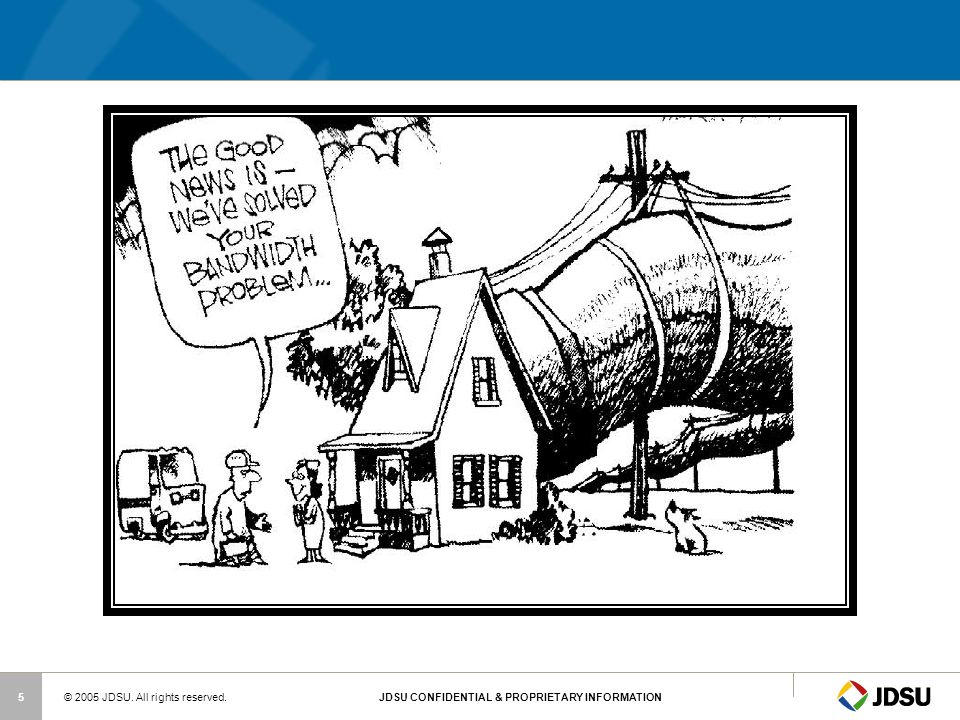


 High-Speed LANs. 2 Introduction Fast Ethernet and Gigabit Ethernet Fast Ethernet and Gigabit Ethernet Fibre Channel Fibre Channel High-speed.>")
 1 Chapter 12 Cross-Layer.>")


