1. Introduction to Algorithms
Rabie A. Ramadan
rabieramadan.org 3
Some of the sides are exported from different sources to clarify the topic

2. Time efficiency of nonrecursive algorithms
General Plan for Analysis
Decide on parameter n indicating input size
Identify algorithm’s basic operation
Determine worst, average, and best cases for input of size n
Set up a sum for the number of times the basic operation is executed
Simplify the sum using standard formulas and rules.

3. Example 1: The Largest Element
T(n) = 1in-1 (1) = n-1 = (n) comparisons

4. Example 2: Element uniqueness problem
T(n) = 0in-2 (i+1jn-1 (1))
= 0in-2 (n-i+1) =
= ( ) comparisons

5. Example 3: Matrix multiplication
T(n) = = ( ) multiplications
Ignored addition for simplicity

6. Plan for Analysis of Recursive Algorithms
Decide on a parameter indicating an input’s size.
Identify the algorithm’s basic operation.
Check whether the number of times the basic op. is executed may vary on different inputs of the same size. (If it may, the worst, average, and best cases must be investigated separately.)
Set up a recurrence relation with an appropriate initial condition expressing the number of times the basic op. is executed.
Solve the recurrence (or, at the very least, establish its solution’s order of growth) by backward substitutions or another method.

7. Example 1 : Factorial: Recursive Algorithm
The stopping condition is n=0
A repetitive algorithm uses recursion whenever the algorithm appears within the definition itself.

8. Example 1: Recursive evaluation of n!
Definition: n ! = 1  2  … (n-1)  n for n ≥ 1 and 0! = 1
Recursive definition of n!: F(n) = F(n-1)  n for n ≥ 1 and
F(0) = 1
Size:
Basic operation:
Recurrence relation:
Note the difference between the two recurrences. Students often confuse these!
F(n) = F(n-1) n
F(0) = 1
for the values of n!
M(n) =M(n-1) + 1
M(0) = 0
for the number of multiplications made by this algorithm n
multiplication
M(n) = M(n-1) (for F(n-1) ) + 1 (for the n * F(n-1))
M(0) = 0

9. Solving the recurrence for M(n)
M(n) = M(n-1) + 1, M(0) = 0 (no multiplication when n=0)
M(n) = M(n-1) + 1
= (M(n-2) + 1) = M(n-2) + 2
= (M(n-3) + 1) = M(n-3) + 3 …
= M(n-i) + i
= M(0) + n
= n
The method is called backward substitution.

10. Example 2: The Tower of Hanoi Puzzle
Towers of Hanoi (aka Tower of Hanoi) is a mathematical puzzle invented by a French Mathematician Edouard Lucas in 1983.
Initially the game has few discs arranged in the increasing order of size in one of the tower.
The number of discs can vary, but there are only three towers.
The goal is to transfer the discs from one tower another tower. However you can move only one disk at a time and you can never place a bigger disc over a smaller disk. It is also understood that you can only take the top most disc from any given tower.

11. Example 2: The Tower of Hanoi Puzzle
Recurrence for number of moves:
M(n) = 2M(n-1) + 1

12. Move Sequence for d = 3 1 2 3 4 5 6 7
7 moves , Right !!!

13. The Tower of Hanoi Puzzle
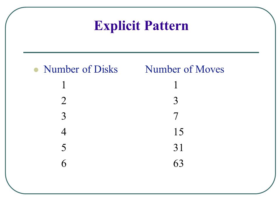
Here's how to find the number of moves needed to transfer larger numbers of disks from post A to post C, when M = the number of moves needed to transfer n-1 disks from post A to post C:
for 1 disk it takes 1 move to transfer 1 disk from post A to post C;
for 2 disks, it will take 3 moves: 2M + 1 = 2(1) + 1 = 3
for 3 disks, it will take 7 moves: 2M + 1 = 2(3) + 1 = 7
for 4 disks, it will take 15 moves: 2M + 1 = 2(7) + 1 = 15
for 5 disks, it will take 31 moves: 2M + 1 = 2(15) + 1 = 31
for 6 disks... ?

14. Explicit Pattern Number of Disks Number of Moves 1 1 2 3 3 7 4 15 5 31
1 1
2 3
3 7

15. Powers of two help reveal the pattern:
Number of Disks (n) Number of Moves
= = 1
= = = = 7
= = 15
= = 31
= = 63

16. Fascinating fact
So the formula for finding the number of steps it takes to transfer n disks from post A to post C is:
2 n - 1

17. Solving recurrence for number of moves
M(n) = 2M(n-1) + 1, M(1) = 1
M(n) = 2M(n-1) + 1
= 2(2M(n-2) + 1) + 1 = 2^2*M(n-2) + 2^1 + 2^0
= 2^2*(2M(n-3) + 1) + 2^1 + 2^0
= 2^3*M(n-3) + 2^2 + 2^1 + 2^0
= …
= 2^(n-1)*M(1) + 2^(n-2) + … + 2^1 + 2^0
= 2^(n-1) + 2^(n-2) + … + 2^1 + 2^0
= 2^n

18. What Is the Important of Fibonacci Sequence?
The Fibonacci numbers:
0, 1, 1, 2, 3, 5, 8, 13, 21, …
The Fibonacci recurrence:
F(n) = F(n-1) + F(n-2)
F(0) = 0
F(1) = 1
F(n) = F(n-1) + F(n-2) or F(n) - F(n-1) - F(n-2) = 0 General 2nd order linear homogeneous recurrence with
constant coefficients:
aX(n) + bX(n-1) + cX(n-2) = 0

19. Chapter 3
Brute Force
Copyright © 2007 Pearson Addison-Wesley. All rights reserved.

20. Brute Force
A straightforward approach, usually based directly on the problem’s statement and definitions of the concepts involved
Examples:
Computing an (a > 0, n a nonnegative integer)= a*a*….*a
Computing n!
Multiplying two matrices
Searching for a key of a given value in a list

21. Brute-Force Sorting Algorithm
Selection Sort Scan the array to find its smallest element and swap it with the first element. Then, starting with the second element, scan the elements to the right of it to find the smallest among them and swap it with the second elements. Generally, on pass i (0  i  n-2), find the smallest element in A[i..n-1] and swap it with A[i]: A[0]   A[i-1] | A[i], , A[min], , A[n-1]
in their final positions
Example:

22. Analysis of Selection Sort
Time efficiency:
Space efficiency:
Stability:
Θ(n^2)
Θ(1), so in place
yes

23. Brute Force - Bubble Sort
Another brute force application to the sorting problem
is to
compare adjacent elements of the list.
and exchange them if they are out of order.
By doing it repeatedly, we end up “Bubbling up” the
largest element to the last position on the list
The next pass bubbles up the second largest element,
and so on until, after n-1 passes, the list is sorted.

24. Brute Force - Bubble Sort
Algorithm BubbleSort (A[0…n-1])
for i ← 0 to n-2 do
for j ← 0 to n-2-i do
if A[j]<A[j+1]
swap A[j] and A[j+1]
The number of times it is executed T(n) depends only on the array’s size and is given by the following sum:

25. Brute-Force String Matching
pattern: a string of m characters to search for
text: a (longer) string of n characters to search in
problem: find a substring in the text that matches the pattern
Brute-force algorithm
Step 1 Align pattern at beginning of text
Step 2 Moving from left to right, compare each character of pattern to the corresponding character in text until
all characters are found to match (successful search); or
a mismatch is detected
Step 3 While pattern is not found and the text is not yet exhausted, realign pattern one position to the right and repeat Step 2

26. Examples of Brute-Force String Matching
Pattern: Text:
Pattern: happy Text: It is never too late to have a happy childhood.

27. Pseudocode and Efficiency
Time efficiency:
Θ(mn) comparisons (in the worst case)

28. Brute-Force Polynomial Evaluation
Problem: Find the value of polynomial
p(x) = anxn + an-1xn-1 +… + a1x1 + a0
at a point x = x0
Brute-force algorithm
Efficiency:
p  0.0
for i  n downto 0 do
power  1
for j  1 to i do //compute xi
power  power  x
p  p + a[i]  power
return p
Θ(n^2) multiplications

29. Polynomial Evaluation: Improvement
We can do better by evaluating from right to left:
Better brute-force algorithm
Efficiency:
Horner’s Rule is another linear time method.
p  a[0]
power  1
for i  1 to n do
power  power  x
p  p + a[i]  power
return p
Θ(n) multiplications

30. Closest-Pair Problem
Find the two closest points in a set of n points (in the two-dimensional Cartesian plane).
Brute-force algorithm
Compute the distance between every pair of distinct points
and return the indexes of the points for which the distance is the smallest.
Draw example.

31. Closest-Pair Brute-Force Algorithm (cont.)
The basic operation of the algorithm is computing the Euclidean distance between two points.
The square root is a complex operation who’s result is often irrational, therefore the results
can be found only approximately. Computing such operations are not trivial. One can avoid
computing square roots by comparing distance squares instead.
Efficiency:
How to make it faster?
Θ(n^2) multiplications
Using divide-and-conquer!

32. Brute-Force Strengths and Weaknesses
wide applicability
simplicity
yields reasonable algorithms for some important problems (e.g., matrix multiplication, sorting, searching, string matching)
Weaknesses
rarely yields efficient algorithms
some brute-force algorithms are unacceptably slow
not as constructive as some other design techniques

33. Exhaustive Search
A brute force solution to a problem involving search for an element with a special property, usually among combinatorial objects such as permutations, combinations, or subsets of a set.
Method:
generate a list of all potential solutions to the problem in a systematic manner
evaluate potential solutions one by one, disqualifying infeasible ones and, for an optimization problem, keeping track of the best one found so far
when search ends, announce the solution(s) found

34. Example 1: Traveling Salesman Problem
Given n cities with known distances between each pair, find the shortest tour that passes through all the cities exactly once before returning to the starting city
Alternatively: Find shortest Hamiltonian circuit in a weighted connected graph
Example: a b c d 8 2 7 5 3 4
How do we represent a solution (Hamiltonian circuit)?

35. TSP by Exhaustive Search
Tour Cost
a→b→c→d→a = 17
a→b→d→c→a = 21
a→c→b→d→a = 20
a→c→d→b→a = 21
a→d→b→c→a = 20
a→d→c→b→a = 17
Efficiency: a b c d 8 2 7 5 3 4
Θ((n-1)!)
Chapter 5 discusses how to generate permutations fast.

36. Example 2: Knapsack Problem
Given n items:
weights: w1 w2 … wn
values: v1 v2 … vn
a knapsack of capacity W
Find most valuable subset of the items that fit into the knapsack
Example: Knapsack capacity W=16
item weight value
$20
$30
$50
$10

37. Knapsack Problem by Exhaustive Search
Subset Total weight Total value
{1} $20
{2} $30
{3} $50
{4} $10
{1,2} $50
{1,3} $70
{1,4} $30
{2,3} $80
{2,4} $40
{3,4} $60
{1,2,3} not feasible
{1,2,4} $60
{1,3,4} not feasible
{2,3,4} not feasible
{1,2,3,4} not feasible
Efficiency:
Θ(2^n)
Each subset can be represented by a binary string (bit vector, Ch 5).

38. Example 3: The Assignment Problem
There are n people who need to be assigned to n jobs, one person per job. The cost of assigning person i to job j is C[i,j]. Find an assignment that minimizes the total cost.
Job 1 Job 2 Job 3 Job 4
Person
Person
Person
Person
Algorithmic Plan: Generate all legitimate assignments, compute their costs, and select the cheapest one.
How many assignments are there? n!

39. Assignment Problem by Exhaustive Search
Assignment (col.#s) Total Cost
1, 2, 3, =18
1, 2, 4, =30
1, 3, 2, =24
1, 3, 4, =26
1, 4, 2, =33
1, 4, 3, =23
etc.
(For this particular instance, the optimal assignment can be found by exploiting the specific features of the number given. It is: )
2,1,3,4

40. Final Comments on Exhaustive Search
Exhaustive-search algorithms run in a realistic amount of time only on very small instances
In some cases, there are much better alternatives!
Euler circuits
shortest paths
assignment problem
In many cases, exhaustive search or its variation is the only known way to get exact solution
The Hungarian method runs in O(n^3) time.