1. Monopoly

4. Introduction Interpretation of monopoly definition
Monopoly or market power
Downward sloping demand curve
Price setting and quantity
Welfare consequences
Sources of monopoly power
Profitable pricing strategies

5. Competition recap

6. Introduction
Brotherhood for the Respect, Elevation, and Advancement of Dishwashers
Impact of achieving goal
SR life better for dishwashers
LR wages of dishwashers decrease by full amount of tips

7. Introduction Why wages bid down by full amount of tips
Who benefits from tipping
Tools for analyzing competitive industry

8. Section 7.1
The competitive firm

9. Competitive Firm Firm sells any quantity wants at going market price
Classic example farm
Small part of market served by each firm
Horizontal demand curve
Products are interchangeable
Buyers can easily buy from another producer

11. Revenue
TR = P X Q
MR ≡ P
MR curve is flat
Coincides with demand curve

13. Firm’s Supply Decision
Produce good until MR = MC
Competitive firm produces a quantity where P = MC
Note: P ≡ MR
Supply curve
MC and supply are inverse functions
Supply curve looks like upward sloping portion of MC curve as long as MC curve upward sloping
SR and LR supply curves exist for the firm

16. Shutdowns and Exits Does the producer want to produce the good?
Two distinctions
Shutdown: firm stops producing the good but still pays fixed costs
Exit: firm leaves the industry entirely and no longer faces any costs
Firms, in SR, can shutdown but not exit
Remains operational if P > AVC
In LR, can exit

18. Short-Run Supply Curve
Firms SR supply curve identical to part of SRMC curve that lies above AVC curve
Shutdown otherwise
Upward sloping due to AC and MC U-shape
Diminishing marginal returns to variable factors of production
Elasticity of supply
Percent change in quantity supplied resulting from a 1% change in price

20. The competitive industry in the short run
Section 7.2
The competitive industry in the short run

21. Competitive Industry in the SR
All firms in industry competitive
SR is period of time in which no firm can enter or exit the industry
Number of firms cannot change
LR is period of time in which any firm can enter or leave the industry
Industry’s SR supply curve
Sum of SR individual firm supply curves
More elastic than individual supply curves

23. Supply, Demand, and Equilibrium
Each firm operates where supply meets demand
Industry equilibrium consequence of optimizing behavior on part of individuals and firms
Intersecting industry wide supply and industry wide demand

24. Competitive Equilibrium
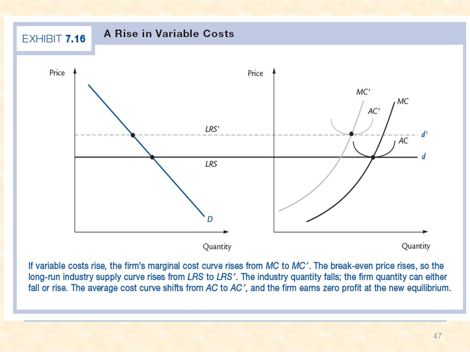
Firms produces where supply (or MC) curve crosses horizontal line at market going price
Increase in FC
Price and quantity remain unchanged
Increase in VC
Raises firms MC curve
Causes some firms to shutdown
Higher market equilibrium price
Firm’s output could go up or down
Increase in industry demand
Increase in firm’s output

26. Change in Fixed Cost Increase in FC
Price and quantity remain unchanged

27. Change in Variable Cost
Increase in VC
Raises firms MC curve
Causes some firms to shutdown
Higher market equilibrium price
Firm’s output could go up or down

29. Change in Industry Demand
Increase in industry demand
Higher market equilibrium price
Increase in firm’s output

31. Industry’s Costs Sum of total cost of all individual firms
To minimize cost of all firms, use equimarginal principle
Insure that MC same for all producers in industry
Automatic because all firms have same price

32. The competitive firm in the long run
Section 7.3
The competitive firm in the long run

33. Competitive Firm in the LR
Some fixed cost in SR become variable cost in the LR
Firms can enter and exit in the LR

34. Profit and the Exit Decision
Profit = TR – TC
Costs includes all foregone opportunities
SR versus LR supply response
Firm LR supply curve more elastic than SR supply curve
Shuts down if price of output falls below average variable cost
Exits if price of output falls below average cost

36. LRMC and Supply Firms operate where P = LRMC
Remain in industry, LR supply curve identical to LRMC curve
Exit decision is made at the point P=AC (note that there is no more fixed cost in the LR)

38. The competitive industry in the long run
Section 7.4
The competitive industry in the long run

39. Competitive Industry in the LR
Firms wishing to enter or exit the market do so in the LR, flatting out the LR supply curve
So unlike the case in the SR, the LR supply curve is a horizontal line.
Important assumption: all firms are identical in costs
Break-even price plays an important role here (1) all firms produce at the break-even price; (2) it determines the level of LR supply curve

41. Zero Profit Condition Economic versus accounting profit
Accounting profit refers to total revenue minus total financial cost
Economic profit refers to accounting profit minus the value of the best foregone opportunity

43. Industry’s LR Supply Curve
All firms identical
Industry supply curve flat at the break-even price
Break-even price and the LR supply
Break-even price (P = AC) at which a seller earns zero profit
LR supply curve identical with part of firm’s LRMC curve lying above LRAC curve

44. Flat LR Supply Curve Flatness based on entry and exit
P < AC, all firms exit
P > AC, unlimited number of firms enter
LR zero profit equilibrium almost never reached
Demand and cost curves shift so often that entry and exit never settles down
Approximation to the truth

45. Equilibrium LR same as SR between firm and industry
Market price determined by intersection of industrywide demand and supply
Firms face flat demand curves at market price
Analysis of changes to equilibrium
Changes in FC
Changes in VC
Changes in demand

49. Application: Government as a Supplier
In SR, government policy to build and operate apartment complex increasing housing
In LR, supply curve does not shift
Determined by break-even price
Number of privately owned apartments withdrawn from the market equals number of apartments built by government

51. Relaxing the Assumptions
Assumption 1: All firms are identical, have identical cost curves
True in industries that do not require unusual skills
Assumption 2: Cost curves do not change as industry expands or contracts
True in industries not large enough to affect input prices
Without these assumptions, all firms do not have the same break-even price

52. Constant Cost
Constant cost industry
Satisfies the 2 assumptions

53. Increasing Cost Increasing cost industry
Break-even price for new entrants increases as industry expands
Assumption 1 violated: Less-efficient firms
Assumption 2 violated: Factor-price effect
LR industry supply curve slopes upward

56. Decreasing Cost Decreasing cost industry
Break-even price for new entrants decreases as industry expands
LR industry supply curve slopes downward

58. Applications
A tax on motel rooms
Tipping the busboy

61. Using the Competitive Model
Fundamentals of competitive analysis
Industry versus firm demand and supply
SR versus LR
Entry and exit decisions

62. Price and output under monopoly

63. Price Pricing operates where MR = MC
MR curves lies everywhere below demand curve

65. Output Lower price to increase output
Monopolist operates on elastic portion of demand curve
Ex. Prices of gasoline, oranges, and music CDs
No supply curve
No going market price

66. Measuring Monopoly Power

67. Welfare
Assumption about same industry wide MC curve for competitive and monopolistic industries
Social welfare loss under monopoly
Marginal value exceeds marginal cost
Monopolist could produce additional good

69. Subsidies and Public Policy
Subsidies for monopolist
Induce monopolist to provide competitive quantity
Arises from “ideal” subsidy
Could encourage inefficient production
Creates price ceilings
Follows rate-of-return regulation

73. Sources of Monopoly Power
Natural monopoly
Industry where AC curve decreasing at point where crosses market demand
Industry survive only if monopolized

75. Sources, cont. Welfare economics Imperfect competition
Monopoly outcome best for some
Imperfect competition
Downward pressure on prices
Innovation

76. Other Sources of Monopoly Power
Patents
Ex. photography
Resource monopolies
Single firm controls productive input
Legal barriers to entry

77. Monopoly, market, and government
This video explains why the concept of monopolies are incompatible with the free market, and actually the result of non-market (government) forces.

78. Price Discrimination Charging different prices for identical items
Ability to prevent resell of low-price units

79. First Degree First-degree Charging each customer most willing to pay
Welfare gains

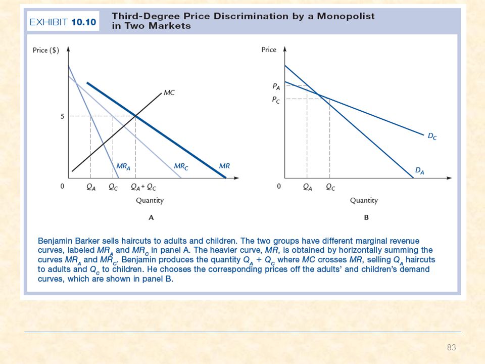
81. Third-Degree Charging different prices in different markets
Groups of consumers identifiable
Different downward sloping demand curve
Producer profit
Production of goods where MR same in both markets and equal to MC
More elastic demand group receives lower price

84. maxy1, y2 (=p1(y1)y1+ p2(y2)y2-c(y1+y2)).
Third-degree: the most common form of price discrimination (student discounts, senior citizens’ discounts). Suppose there are two groups of people and there is no resale. Then the monopolist’s profit maximization problem becomes
maxy1, y2 (=p1(y1)y1+ p2(y2)y2-c(y1+y2)).
Hence FOC becomes
MR1(y1)=MC(y1+y2)=MR2(y2).

85. Since MR1(y1)=p1(y1)[1-1/|1|] and MR2(y2)=p2(y2)[1-1/|2|], hence p1>p2 if and only if |1|<|2|. The market with lower absolute value of elasticity has a higher price. Quite sensible since elasticity measures how sensitive the group is to price changes.
There are some other often-observed practices used by firms with monopoly power.

86. Second-degree: also known as non-linear pricing since the price per unit of output is not constant, but depends on how much you buy. The monopolist can offer different price-quantity packages so that the consumers can self select.
Note that the low-end consumer’s package is distorted so that the high-end consumer will not choose the low-end package.

87. Fig. 25.3

88. Compared to perfect price discrimination, without high-end, low-end is offered higher quantity but still ends up with zero surplus. Without low-end, high end gets zero surplus, now gets positive surplus and the quantity offered is the same.
Applying this to air travels, by offering a downgraded product, the airlines can charge the consumers who need flexible travel arrangements more for their tickets.

89. Many many examples of PD
Coupons, rebates, free delivery, coffee lids……
The spirit of PD – to offer lower prices to customers who are more sensitive to price. There is no point to offer coupons if everyone redeemed them, and there is no point to coupons if only a random set of customers redeemed them.
Note: almost everything that appears to be price discrimination admits at least one alternative explanation. For example, coupon clippers temp to go shopping when the shop is not crowded.

90. Pricing strategies by monopolist: versioning
Versioning is a practice of offering an inferior product to charge differently for different customers. For example, hardcopy and paperback of the same book. Another example is the same printers designed to print slower deliberately.
Strictly speaking, versioning should not be considered as a form of PD in some cases as products involved are different.

91. Pricing strategies by monopolist: Two-Part Tariff
First part
Entry fee allows purchase of goods or services
Meaning of tariff

92. Pricing strategies by monopolist: Two-Part Tariff
Second part
Customers are charged maximum willing to pay
Charge competitive price as long as no difference in consumers
Charge low initial fee and high usage fee

94. Pricing strategies by monopolist: Two-Part Tariff
By implementing the two-part tariff, a monopoly firm can produces at the competitive market level, enhancing the efficiency.
Examples
Clubs that charge a member fee and an usage fee
Health insurance – copayment increases efficiency.

95. Pricing strategies by monopolist: Bundling
packages of related goods are often offered for sale together: software suite (word processor, spreadsheet, presentation tool), cosmetic products, etc.
Bundling may be cost saving or it may be due to complementarities among the goods involved. But there can be reasons involving consumer behavior. Consider the following example. Assume the marginal cost of producing is zero.

96. Type of consumers
word pro spreadsheet A B
Suppose the willingness to pay for the bundle is the sum. If each item is sold separately, then revenue will be 400. If instead bundling two goods together, can get the revenue of 440. In other words, the dispersion of willingness to pay may be reduced.