CHAPTER ONE The Economic Problem.

CHAPTER ONE The Economic Problem

What Is Economics ? Definition: Economics is defined as : The study of the use of scarce resources to satisfy unlimited human wants . Another definition of Economics : It is the science of choice . Therefore, it is the science that explains the choices we make .

The Aim of Economics To help the people obtain the greatest possible satisfaction out of the resources at their disposal, which means to do the best they can with what they have .

What are the Society’s Resources ?
1. Natural Resources such as Land, Forests, and Minerals . 2. Human Resources both mental and Physical . 3. Manufactured aids to production such as tools, machinery, and buildings .

What is Scarcity ? Scarcity means that we do not have enough of everything , including time, to satisfy our every desire . Scarcity exists because human wants always exceeds what can be produced with the limited resources available . Scarcity implies that we must make choices .

Choice Choice is a trade off , which means that we give up something to get something else . Every choice involve a cost .

It is the best alternative given up or forgone.
The Opportunity Cost It is the best alternative given up or forgone. It is the action that you choose not to do .

Example What is the opportunity cost of attending a 3 hours lecture in economics ? For a Jogger is the forgone 3 hours of exercise . For early sleeper is the forgone 3 hours in bed . And so on .

Example 2 Consider the choice that must be made by your little brother who has SR 5 to spend and who is determined to spend it all on candy. Assume there are only two kinds of candy that he can buy ( Bubble Gum which sells for SR 0.50 each ) and ( Chocolates which sells for SR 1.00 each ) . What are the attainable combinations ?

Attainable Combinations
Bubble Gums Chocolates Total cost SR 5 SR 5 SR 5 SR 5 SR 5 SR 5

Example 2 - continue After careful thought , your brother has almost decided to buy 6 bubble gums and 2 chocolate, But at the last moment he decided that he must have 3 chocolates . What will it cost to get this extra chocolate ? The answer is two bubble gums, so he has to give up 2 bubble gums to get one more chocolate . The 2 bubble gums is called by economists as the opportunity cost of the third chocolate.

Graphically 10 9 8 7 6 5 4 3 2 1 1 2 3 4 5 6 7 8 9 10 unattainable
Graphically unattainable attainable

Production Possibilities
Production: Is the conversion of Natural, Human , and Capital resources into goods and services . Production Possibility Boundary: Makes the boundary between production level that can and can not be attained .

Example Assume the following : 1. There is only one producer ( Ahmed )
2. There are only two goods to be produced ( Corn and Cloth ) 3. Ahmed can work 12 hours each day . So, the amount of Corn and Cloth that Ahmed can produce depends on how many hours he devotes to producing them .

In addition you are given the following Table # 1
Hours worked Corn Grown Cloth produced per day pound per month Yards per month 3 either or 6 either or 9 either or 12 either or Calculate Ahmed’s Production boundary ?

Ahmed’s Production Possibility Boundary
Possibility Corn Cloth (pound per month) (Yard per month) a and b and c and d and e and

Note: Points on the boundary is always better than points inside the boundary . Points on the boundary ( a,b,c,d, and e ) represent full and efficient use of society’s resources . While points inside the boundary represent either inefficient use of resources or failure to use all the available resources .

Four Key Economic Problems
Whatever the economic system, most problems studied by economists can be grouped under 4 main headings : 1. What is Produced and How ? 2. What is consumed and by whom ? 3. Why are Resources sometimes idle ? 4. Is production capacity growing ?

I. What is Produced and How ?
The allocation of scarce resources among alternative uses determines the quantity of various goods that are produced. Because resources are scarce, it is desirable that they be used efficiently . If resources are used efficiently, than at which point on the boundary will production take place ? .

What is Consumed and by Whom ?
Will the economy consume exactly the same goods as it produces ? Or , will the country’s ability to trade with other countries permit the economy to consume a different combination of goods ? Who consume the goods and services produced depends on the income that people earns .

III. Why are Resources sometimes idle ?
When an economy is in a recession some resources such as labor, factories and equipment, and raw materials are idle. Why are resources sometimes idle ? And should government worry about such idle resources ?

IV. Is productive capacity growing ?
Growth in production capacity can be represented by an outward shift of the production possibility boundary . If an economy’s capacity to produce goods and services is growing, combinations that are unattainable today will become attainable tomorrow . Growth makes it possible to have more of all goods .

Alternative Economic Systems
There are 3 types of economic systems . These are : 1. Traditional Systems . 2. Command Systems . 3. Market Systems .

I. Traditional Systems A traditional economy is one in which behavior is based primarily on Traditions, Customs , and Habits . Example : Young men follow their father’s occupations . Women do what their mother did . So , there is little change in the patterns of goods produced from year to year .

II. Command Systems Economic behavior id determined by some central authority ( Government ) which make most of the necessary decisions on : What to prodce ? How to produce it ? Who will gets it ? Such economies are characterized by the Centralization of Decision Making . Example : China and Cuba .

III. Market Systems ( Free-Market economy )
In such an economy, decisions relating to the basic economic issues are decentralized . Decisions are made by individual producers and consumers .

Mixed Systems Economies that are fully traditional or fully centrally planned or wholly free-market are pure types that are useful for studying basic principles. But in practice, every economy is a mixed economy in the sense that it combine significant elements of all three systems in determining the economic behavior .

Ownership of Resources
Economies differ as to who own their productive resources. Example : Who owns a nation’s farms and factories Who owns a nation’s coal,mines,& forests ? Who owns a nation’s railways,airline, hotels, etc. ?

Private-Ownership Economy
The basic raw materials, the productive assets of the society, and the goods produced in the economy are pre-dominantly privately owned. Example : the U.S.A. System .

Public-Ownership Economy
Is one in which the productive assets are predominantly publicly owned . Example : China and Former Soviet Union

CHAPTER 4 Demand and Supply

In this Chapter 1. We need to understand what determines the demand for a particular product ? 2. We will also study what determine the supply of a particular product ? 3. We will see how demand and supply together determine the price of a product and the quantity that are exchanged in the market ?

The Demand What determine the demand for a product ? To answer this question , we have first to distinguish between two terms : 1. Quantity Demanded 2. Demand

Quantity Demanded Is the total amount of any particular good or service that the consumer wish to purchase in some time period for a given price .

The Term Demand Refers to the entire relationship between the quantity demanded of a product and the price of that product . Therefore : The quantity demanded represent a single point on the demand curve .

The Law of Demand A basic economic assumption is that :
“ The price of any good and the quantity demanded of that good are negatively related, other things being equal . “ Therefore : The lower the price of a good, the higher the quantity demanded of that good . And The higher the price, the lower the quantity demanded .

The Law of Demand-continue
This negative relationship between the price and the quantity demanded is called “ The Law of Demand “ . This relationship can be shown by : 1. Demand Schedule or 2. Demand Curve .

The Demand Schedule The Demand Schedule is a table that shows the quantity demanded of a product at different prices . The Demand curve is a graphical representation of the demand Schedule .

Example Price of Carrots Quantity demanded
( per ton ) ( in thousands of tons) $

Factors that influence the Quantity Demanded
1. The product’s own price . 2. The prices of related products . 3. The Income . 4. The Population . 5. The Preferences or Tastes . 6. The expected future prices .

Quantity Demanded and the price
How the quantity demanded of a product changes as its price change ?

Change in Quantity Demanded
If we assume that the price of a product may change, while other factors that influence the quantity demanded remain constant, then that causes a movement along the demand curve . Therefore, a movement along the demand curve shows a change in quantity demanded.

Change in Demand If the price of the product is held constant, and other factors changes such as Income , population, preferences, etc. , that will cause a shift in the demand curve . Therefore, a shift in demand curve to the right or to the left shows a change in demand.

Determinants of Demand
The determinants of demand are what cause consumers to change their view of how much they will buy of a given good or service at all possible prices that could be charged for it. These determinants depends on the good in question .

Some Determinants of Demand
1. Consumer Income 2. Population ( # of consumers in the market) 3. Prices o related products 4. Preferences or Tastes . 5. Expected Future Prices .

Consumer Income Normally as consumers’ income increases, they tend to purchase more goods and services . Therefore, If an individual consumer purchase more of a good when his income increases , that good is said to be Normal good. And if the consumer purchase less of a good when his income increases, that good is said to be an inferior good .

Consumer Income-continue
For a Normal good : an increase in income will shift the demand curve to the right. And a decrease in income will shift the demand curve to the left . For an inferior good : an increase in income will shift the demand curve to the left . And a decrease in income will shift the demand curve to the right .

Prices of related Products
The relation between the quantity demanded of a good and the price of related good depends on whether the two goods are substitutes or complements .

Substitute Goods Substitute goods are goods that can be used in place of other goods . Example : Tea and Coffee or Pepsi and Coke A good will be substituted in place of other good if it become relatively cheaper than other good.

Substitute goods - continue
For substitute goods , there is a positive relation between quantity demanded of one product and the price of other product . Example : As price of coffee rises, the quantity demanded of tea rises . And As price of coffee falls, the quantity demanded of of tea falls .

Complements Are products that are tend to be used jointly or together . Example : Car and Gasoline Computer and Printer Tea and Sugar A fall in price of complementary product will shift a product demand curve to the right which means more will be purchases at each price .

Complements - continues
A rise in price of complementary product will shift the demand curve of the product to the left. Therefore, there is a negative relationship between the price of complementary product and the quantity demanded of the product .

Population Demand also depends on the size of the population or # of consumers in the market : The larger the population, the greater is the demand for all goods and services , and that shift the demand curve to the right . And the smaller the population, the smaller is the demand for all goods and services, so the demand curve will shifts to the left .

Preferences or Tastes A change in taste in favor of a product will increase the demand for that product, and shift the demand curve to the right . And a change in taste against the product will decrease the demand for that product and shift the demand curve to the left .

Expected Future Prices
If the consumers expect that prices of the product will rise in the future, they will increase their demand for the product today. This will shift the demand curve of that product to the right . And if the consumers expect that prices of the product will fall in the near future they will decrease their demand today. This will shift the demand curve of that product to the left .

Supply Here, we need to distinguish between Quantity Supplied and Supply . Quantity supplied of a product is : The amount that the producer plan to produce and sell during a given time period at a particular price .

Supply Refers to the entire relationship between the quantity supplied and the price of the product .

Determinants of the Quantity Supplied
1. The price of the product 2. Prices of resources used to produce the product . ( input prices ) 3. Technology 4. The number of suppliers 5. Prices of related goods produced 6. Expected future prices

1. The quantity supplied & the price
The Law of Supply: A basic economic assumption states that : For any product, the price of the product and the quantity supplied are positively related . Which means : The higher the price, the greater is the quantity supplied .

Note This positive relationship between the price and the quantity supplied can be shown by : 1. Supply Schedule , or by 2. Supply Curve

Supply Schedule It is a table that shows the positive relationship between quantity supplied and the price of the product , other things being equal .

Example Supply Schedule of X Price of X Quantity Supplied of X
SR ,000 ,000 ,000 ,000 And so on .

Supply Curve Is a graphical representation of the supply schedule .

Change in Quantity Supplied
A change in the price of the product, holding other factors constant, will cause a change in quantity supplied in the same direction as the change in the price . The change in quantity supplied as a result of change in price will cause upward or downward movement along the supply curve

Change in Supply Holding the price of the product constant, a change in any of the following factors will change the supply and cause a shift in the supply curve : 1. Number of suppliers 2. Prices of related goods produced 3. Expected future prices . 4. Prices of resources used in production

The Determination of Price
How the two forces of the market (the Demand & Supply ) interact to determine the price of the product in the market ? To answer the above question let us look at the following schedule

Demand & Supply Schedule
Price of X Quantity Demanded Quantity Supply SR

Note When actual price is above the equilibrium price, then Quantity supplied > Quantity demanded , and that will create excess supply , which put pressure on prices to go down . When actual price is below the equilibrium price, then Quantity demanded > Quantity supplied, and that create excess demand , which put pressure on prices to go up .

Note The price at which quantity demanded exactly equals to quantity supplied is called “ Equilibrium price or Market Clsearing Price “ and and price where Quantity demanded does not equal Quantity supplied is called Disequilibrium Price .

1. A rise in demand 2. A fall in demand 3. A rise in supply
Laws of Demand & Supply 1. A rise in demand 2. A fall in demand 3. A rise in supply 4. A fall in Supply

1. A rise in demand If there is an increase in demand, that will shift the demand curve to the right, and increase both the equilibrium price and the equilibrium quantity exchanged.

2. A Fall in Demand If there is a fall in demand then that will shift the demand curve to the left, and decrease both the equilibrium price and equilibrium quantity exchanged.

3. A rise in Supply A rise in supply will shift the supply curve to the right and that will decrease the equilibrium price and increase the equilibrium quantity exchanged .

4. A Fall in Supply A fall in supply causes a shift in the supply curve to the left and that will increase the equilibrium price and decrease the equilibrium quantity exchanged .

CHAPTER 5 Elasticity

Price Elasticity of Demand
It measures the responsiveness of quantity demanded of a product to the change in the market price . Therefore : PE = % change in quantity demanded % change in the price

Arc Elasticity Measures the average responsiveness of quantity demanded to the change in the price over an interval of demand curve . Therefore , PE PE = Q2 – Q / P2 – P1___ (Q1 +Q2) / (P1 +P2) / 2 PE = Q2 – Q X (P1+P2)/2 . (Q1+Q2)/ P2 – P1

Example Given the following demand schedule , Calculate the Arc price Elasticity of demand Price Quantity demanded $ PE = 20 – X (20+40)/ = 2 40 – ( )/2

Point Elasticity It measures the responsiveness of Quantity demanded to the change in price of a particular product at a particular point on the demand curve .

Example Given the following demand schedule, Calculate the Point Elasticity of demand. Price of X Quantity demanded of x $ PE = 20 – X = 40 –

The Numerical Value of Elasticity
The numerical value of elasticity vary from Zero to infinity . Therefore : 1. PE = Perfectly inelastic demand < PE < 1 inelastic demand 3. PE = unit elastic demand 4. PE > elastic demand 5. PE = infinity Perfectly elastic demand

Perfectly inelastic demand when PE = 0
When PE = 0 it means that quantity demanded does not respond at all to the change in the price of the product . Example : Price Quantity demanded $ PE = 100 – 100 X (20+40)/2 = X 30 = 0 ( )/

Inelastic Demand 0<PE<1
When < PE < inelastic demand This means that : % change in quantity < % change in the price Example : Price of x Quantity demanded of x $ PE = 80 – X ( )/2 = 0.33 40 – ( )/2

Unit elastic demand , PE = 1
When PE = 1 , we have unit elastic demand This means that : % change in quantity = % change in price Example : Price Quantity demanded $ PE = 50 – X ( )/2 = 1 ( )/2

Elastic Demand , PE > 1 When PE > 1 , we have elastic demand
This means that : % change in quantity > % change in the price Example : Price of x Quantity demanded $ PE = 20 – X ( )/2 = 2 40 – ( )/2

Price elasticity and change in Total Revenue ( or total expenditure )
How does total revenue react to a change in the price of a product ? The response of total revenue depends on the price elasticity of demand which means it depends on whether the demand is elastic, inelastic , or unit elastic ?

If the Demand is elastic, PE>1
In this case , the price and total revenue are negatively related . Therefore : A fall in the price , will increase total revenue A rise in the price, will decrease total revenue Example : Price Quantity Total $ $ 2000 PE = 2

If the Demand is inelastic , PE <1
If the demand is inelastic , PE < 1 , then Price and total revenue are positively related, which means : A fall in price , will decrease total revenue , and A rise in price, will increase total revenue Example : Price Quantity Total revenue $ $ 2000 PE = 0.33

If the Demand is Unit elastic , PE=1
When the demand is unit elastic, PE = 1 ,then Total revenue will not be changed ( constant ) which means : As price rises or falls , total revenue remain unchanged . Example : P Q TR $ $ 2000 PE = 1

Determinants of The Price Elasticity of Demand
The main determinant of elasticity of demand is the availability of substitute A product with close substitute tend to have elastic demand . While a product with no close substitute tend to have inelastic demand .

Other Demand Elasticity
1. Income Elasticity of Demand 2. Cross Elasticity of Demand

Income Elasticity of Demand,Ei
This elasticity measures the responsiveness of demand to a change in income . EI = % change in Quantity Demanded % change in Income Where EI = Income elasticity The income elasticity could be positive or negative.

Positive Income Elasticity , EI>0
Goods with positive income elasticity are called “ Normal Goods . Therefore , for Normal Good As income rises , consumption rises . And As income falls , consumption falls . Example : Income Quantity Demanded $ EI = X = = 1.3

Example 2 Income Quantity Demanded $ 1000 100 3000 200
$ EI = X = = 0.67

Negative Income Elasticity, EI<0
Goods with negative income elasticity are called “ Inferior Goods “ . Therefore for Inferior goods : As income rises , consumption will falls and As income falls , consumption will rise .

Example Income Quantity Demanded $ 1000 100 3000 60
$ EI = X = Since EI = < 0 negative EI , therefore X = an inferior good .

Cross Elasticity of Demand
This elasticity measures the responsiveness of demand to the change in the price of another product. It is defined as : E x y = % change in quantity demanded of X % change in the price of Y E x y = Q2 – Q1 X ( P y2 – Py1) /2 P2 – P (Q x2 – Q x1) /2 The Cross elasticity could be positive or negative

Positive Cross elasticity, Exy > 0
If the Cross elasticity is positive , then Both goods ( X and Y ) are Substitutes If the Cross elasticity is negative , then Both goods ( X and Y ) are Complements

Example Price of Coal Quantity demanded of Oil $ 10 100 20 300
$ E xy = X = = 1.5 Since E xy = 1.5 > 0 Positive Cross elasticity Therefore, X and Y are Substitutes .

Example 2 Price of Car Quantity demanded of Gasoline SR 50,000 100,000
30, ,000 Exy = 100,000 X 40,000 = - 20, ,000 Since Exy = < 0 , therefore, Car and Gasoline are complements .

Elasticity of Supply, Es
This elasticity measures the responsiveness of the quantity supplied to a change in the product’s price and it is defined as : Es = percentage change in quantity supplied percentage change in the price The elasticity of supply range between zero and infinity , so 0 < Es < infinity

What Determines the Elasticity of Supply ?
1. The ability of the firm to shift the resources from the production of other commodities to the one whose price has risen . 2. Cost behavior : If cost of production rises rapidly as output rises, then there is no incentive to expand the production , so supply will be less elastic ) . But if cost rises only slowly as production increases, then a rise in price will stimulate a large increase in quantity supply, so the supply will be more elastic .

Short-run and Long-run market adjustment
Shift in demand or supply have different effects on equilibrium price and quantity depending on the degree of price elasticity . Shift in Supply: In the short-run , when demand is relatively inelastic, a shift in supply leads to sharp change in equilibrium price, but to only a small change in equilibrium quantity . But, in long-run , demand is more elastic , so shift in supply curve results in small change in equilibrium price and large change in quantity.

Shift in Demand In the short-run, when supply is relatively inelastic, a shift in demand leads to sharp change in equilibrium price , but only to a small change in equilibrium quantity . However, in the long-run, when supply is more elastic than short-run, a shift in demand leads to a small change in equilibrium price , but to a large change in equilibrium quantity .

Demand and Supply in Action
CHAPTER 6 Demand and Supply in Action

Government Controlled Prices
In some cases , government fix the prices of some products in the market . Government price controls are policies that attempt to hold the prices at some disequilibrium value . Some controls , hold the market price below its equilibrium value. This create a shortages . Other controls, hold price above equilibrium. This create a surplus at the control price .

Quantity Exhanged At any disequilibrium price, we know that the quantity exchanged is determined by the lesser of quantity demanded or supplied. Therefore : For price below equilibrium price , quantity exchanged will be determined by the supply curve. For the prices above the equilibrium price, the quantity exchanged is determined by the demand curve .

Floor Price It is the minimum price that can be charged for a product . The floor price that is set at or below the equilibrium price has no effect because the equilibrium price remain attainable. But, if the floor price is set above the equilibrium price , it is said to be binding or effective .

Note The effective floor price leads to excess supply.
Either unsold surplus will exist or some one must enter the market and buy the excess supply .

Ceiling Price Is the Maximum price at which certain good or service may be sold . If the ceiling price is set above the equilibrium price , it has no effect because the equilibrium price is attainable . But , if ceiling price is set below the equilibrium price , it is said to be effective or binding .

Note The effective ceiling price will create excess demand or shortages and this invite what is called “ Black Market : where goods are sold at illegal price ( the price is higher or lower than the controlled price ) .

Rent Control : A case study of price ceiling
Rent controls are just special case of price ceiling . Here, we need to distinguish between short-run and long-run supply or rental accommodation .

Short-run Supply The short-run supply for Housing is quite inelastic because it takes years to plan and build new apartments . Therefore, the supply curve in short-run is perfectly inelastic , which means : An increase or decrease in demand will cause rent to change in short-run , but there is no change in quantity supplied.

Long-run Supply The Long-run supply curve of rental housing is highly elastic because : If the return on investment in new housing rises significantly above the return on comparative investment , there will be flow of investment funds into the industry of new rental housing. And if the return on investment in new housing fall below what can be earned on comparative investment , the fund will go elsewhere.

The effect of rent control in short and long run
Rent Quantity Quantity Surplus + demanded supply or shortage - $ Assume we have ceiling price at $ 30

Note If the ceiling rent is set below the equilibrium rent that will cause shortages in both the Short-run as well as in the Long-run, but the shortages in the Long-run will be greater because the supply curve in the long-run is more elastic.

Who gain and Who loss from rent control ?
Tenants in rent control accommodations are the gainers . While Landlords and potential future tenants are the losers . Note: Chapter 6 up to page 121 only Up to ( Agriculture & Farm problem)

CHPTER 7 Consumer Behavior

Main Points In this chapter, we will discuss :
Marginal Utility & consumer choice Utility Schedules & Graphs Maximizing Utility Marginal & Total Utility Derivation of consumer Demand curve Consumer Surplus Income & Substitution Effects .

Marginal Utility & Consumer Choice
Consumer choice is fundamental to market economies . Consumers make all kinds of decisions Economists assume that consumers are motivated to maximize their utility . How the consumer make decision based on utility maximization ?

Definition of Utility Utility is defined as follows :
“ It is the satisfaction that the consumers drive from the goods and services that they consume .

Total Utility Is the full satisfaction resulting from the consumption of that product by the consumer .

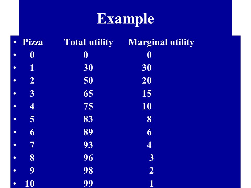
Marginal Utility It is the change in satisfaction resulting from consuming one more unit of the product . Or It is the additional utility derived from consuming one more unit of the product. MU = Change in total utility Change in number of unit consumed

Example Pizza Total utility Marginal utility 0 0 0 1 30 30 2 50 20

Diminishing Marginal Utility
The basic hypothesis of utility theory is called “ Law of diminishing Marginal utility “ which means that : The utility that may any consumer drives from successive units of particular product diminishes as total consumption of that product increase, holding consumption of all other products constant

Maximizing Utility [ equilibrium]
How can a household adjust its expenditure so as to maximize its utility ? The condition for utility maximization is : M U x = M U y P x P y Where M U x = marginal utility per dollar P x spent on X

Equilibrium Condition
Alternatively, we can write the equilibrium condition as follows : M U x = P x . M U y P y MU x = Relative marginal utility of both MU y goods X and Y P x = Relative prices of both goods P y X and Y

Example Assume an individual who spend his income on two goods ( X and Y ) has an income of $ Assume also that the price of X = $ 60 and the price of Y = $ 30 . In addition you are given the following data : Q x TU x Q y TU y Required : How many units of X and Y this consumer should consume to maximize his utility ?

The Answer Q x TU x MU x MU x Q y TU y MU y MU y P x P y
He should consume 2 x and 6 y to maximize his utility

Income and Substitution Effects
How does the household react to a change in the price of one good ? A fall in the price of one good affects the consumer in two ways : 1. Relative price change : This provide an incentive to buy more of the good which its price has fallen . 2. The household real income increases .

Example Assume the following : Income = $ 360 Price of X = 12
Price of Y = 6 Relative price of X to Y = $ 12 = 2 6 What will happen if price of X fall to $ 6?

Substitution Effect Is the change in quantity demanded as a result of a change in relative prices with real income held constant .

Income Effect Is the change in quantity demanded as a result of a change in real income .

Note 1. The substitution effect is always negative .
2. Income effect could be positive or 3. Goods with positive income effect are called “ Normal goods “ 4. Goods with negative income effect are called : “ Inferior goods “

Note 5. Normal goods always have downward demand curve .
6. Inferior goods may have downward or upward demand curve . 7. Inferior goods with downward demand curve is called : Non-Giffen goods “ 8. Inferior goods with upward demand curve is called “ Giffen goods “

Note If substitution effect > negative income effect
Then that good is called Non-Giffen goods . If substitution effect < negative income effect then that good is called Giffen good .

Production and Cost in the Short-run
Chapter 8 Production and Cost in the Short-run

Note In this chapter we will talk about
- production of goods & services by the firms . - How we determine or measure the cost as well as the profit of the firms .

Short-run Is a period of time where at least one or more of the input factors used in production can not be changed ( Fixed). Therefore, in short-run, we have 1. Fixed inputs factors . 2. Variable inputs factors .

Long-run Is a period of time where all factors of production used by the firm can be changed ( Variable )

Profit Maximization Economists usually assume that firms try to make their profit as large as possible which means to maximize their profit. Firms seek profit by producing and selling commodities . All production can be accounted for by the service of 3 kinds of inputs called Factors of production .

Factors of Production 1. Land 2. Labor 3. Capital
The value of these inputs is called “ Cost “

Measurement of Cost There are two ways of measuring the cost
1. Historical cost [ cost of purchased and hired factors ] 2. Opportunity cost : which is the cost of all inputs used in production whether it is purchased, hired, or imputed cost .

It is the value of resources at prices actually paid for them .
Historical Cost It is the value of resources at prices actually paid for them . It is the value of all purchased and hired input factors .

Opportunity Cost It is the cost of the best alternative given up .
It is the cost of each input used in production whether it is purchased, hired , or imputed cost. Opportunity = cost of purchased + imputed cost cost and hired factors = ( Explicit cost ) + ( Implicit cost)

Imputed cost ( Implicit cost )
It is the cost of inputs used in production which is neither purchased nor hired . It is the cost of inputs which its uses does not require payment to anyone outside the firm. Example: The owner’s services to the firm (time and effort ) . The owner’s investment in the firm .

The meaning of Economic Profits
Profit = Revenue – Cost Since we have different measurement of cost , we also have different measurement of profit each based on different measurement of cost . Accounting = Revenue – Historical cost profit Economic = Revenue – opportunity profit cost

Note When Revenue = opportunity cost , then
Economic profit is = 0 this is called Normal profit . When Economic profit > 0 the firm is earning more than the normal profit . When economic profit < 0 the firm is earning less than the normal profit .

Example Assume you are given the following data for a firm .
Revenue from sale SR 300,000 Cost of goods sold SR 150,000 Utilities & other services SR 20,000 Wages ( hired ) SR 50,000 Depreciation SR 22,000 ; Bank interest In addition you know that the owner of the firm invested SR 115,000 of his own money in the firm and worked 1000 hours during the year in his firm where the rate per hour is SR 40 and rate of interest is 10% . Calculate the Accounting profit and the Economic Profit ?

Accounting Profit = Revenue – Historical cost
Revenue SR 300,000 Less: Historical cost : cost of goods sold SR ,000 Utilities & other services 20,000 Wages ( hired ) ,000 Depreciation ,000 Bank interest , ,000 Accounting Profit SR ,000

Economic Profit = Revenue – Opportunity cost
Revenue SR 300,000 Less : Opportunity cost: Cost of goods sold SR 150,000 Utilities & services ,000 Wages ( hired ) ,000 Bank interest ,000 Fall in value of assets ,000 Owner’s salary ,000 Interest on owner’s money 11, ,500 Economic Profit SR ,500

Short-run Production Function
Give us the relationship between the inputs used in production and the output produced. The short-run production can be described by three ways : 1. Total product curve 2. Average product curve 3 . Marginal product curve

Example Assuming a firm using only 2 inputs
( Labor & capital ) where Labor is the variable factor and capital is a fixed factor . In addition you are given the following data : Labor Capital Output

Total Product , TP Is the total amount that is produced during a given period of time . Total product will change as more or less of the variable input factor is used with the given amount of the fixed factor

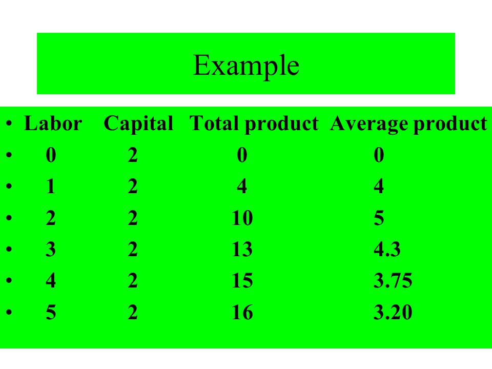
The Average Product , AP AP = TP = Q L L
Is the total product divided by # of units of the variable input used in production. AP = TP = Q L L Where : AP = Average product TP = Total product L = Labor

Example Labor Capital Total product Average product 0 2 0 0 1 2 4 4

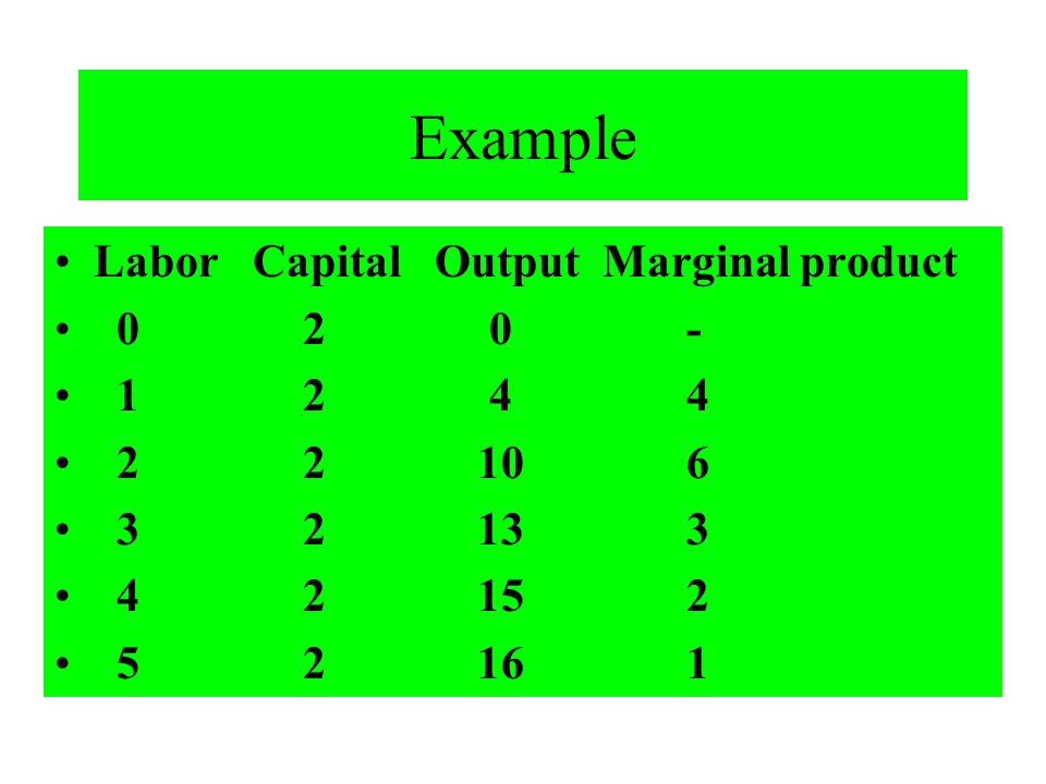
Marginal Product , MP Is the change in total product (output ) resulting from the use of one more unit of the variable input factor . MP of L = change in total product change in Labor

Example Labor Capital Output Marginal product 0 2 0 - 1 2 4 4 2 2 10 6

Relationship between AP and MP
When MP > AP ……. AP is rising When MP < AP ……. AP is falling When MP = AP …. AP is at its Maximum The point at which AP is at its maximum is also called “ point of diminishing AP “

Short-run Variation in Cost
How the firm’s cost vary as its varies its output ? First let us have a brief definition of several cost concept such as : Total cost ; Total fixed cost ; Total variable cost ; Average total cost ; Average fixed cost ; Average variable cost ; and Marginal cost .

Total Cost , TC Is the sum of the cost of all input used in production . Total cost is divided into two parts Total fixed cost and total variable cost . Therefore : TC = TFC + TVC

Total Fixed Cost , TFC This cost does not change as output changes .
It is independent of the level of output . It is also called “ overhead cost “ or “ unavoidable cost “

Total Variable Cost , TVC
This cost vary with the level of output . It is the cost of all variable input used in the production . It is also called “ Direct cost “ or “ avoidable cost “ .

Q Or ATC = AFC + AVC Average Total Cost , ATC
It is the total cost per unit of output . ATC = TC Q Or ATC = AFC + AVC

Marginal Cost ; MC Is the increase in total cost resulting from a unit increase in output . It is also called “ incremental cost . MC = change in total cost change in output

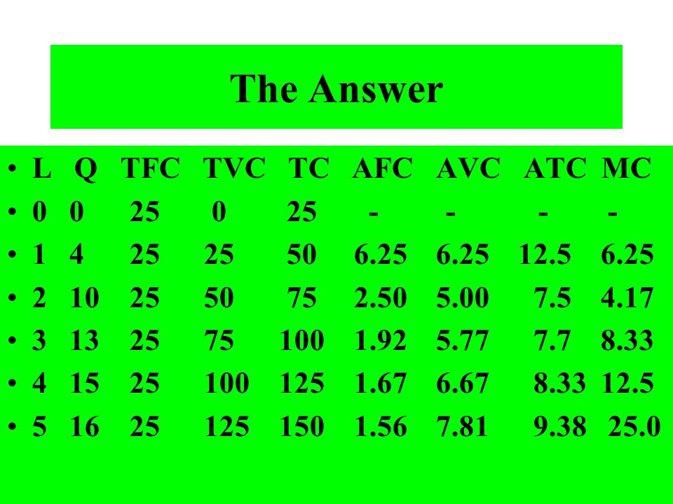
Example Assume that TFC = $ 25 per day , and a worker cost $ 25 per day . Assume Labor is variable input. In addition you are given the following data : Labor Output Required: Calculate TFC ; TVC ; TC ; AFC ; AVC ; ATC ; and MC

The Answer L Q TFC TVC TC AFC AVC ATC MC 0 0 25 0 25 - - - -

Notes 1. TFC is constant at $ 25 regardless of the level
of output , so it has a horizontal cost curve . 2. TVC and TC both increase as output rises . 3. The vertical distance between TC and TVC curves is equal to TFC . 4. AFC decreases as output rises . 5. AVC and ATC both take the U-shape which means they first decrease , reach a minimum and then rises .

Production and Cost in the Long-Run
Chapter 9 Production and Cost in the Long-Run

In the Long-Run All input factors are variables. No Fixed factors .
There are different ways to produce the given output .

Capital Intensive Method
Using more capital and less labor

Labor Intensive Method
Using more labor and less capital

Profit Maximization & Cost Minimization
To maximize the profit in the long-run The firm should select the method that produces its output at the lowest cost possible . This implication is called “ Cost Minimization”

What can the firm do in the long-run to make its cost as low as possible?
Choice of Factor Mix : The firm should substitute one factor (ex. capital) For another factor ( ex. Labor) as long as the Marginal product of one factor per dollar is greater than the marginal product of the other factor per dollar expended on it .

Condition for Cost Minimization
MP K = MP L P K P L Where MP K = marginal product of capital per dollar P K spent on capital MP L = marginal product of labor per dollar spent P L on labor

Note Whenever the two sides of the equation are not equal, there are possibilities to Substitute one factor for another to minimize the cost of production .

Example Therefore, the firm should use more capital and less labor .
If MP K = last dollar spent on K P K added 10 units to the output . And If MP L = last dollar spent on P L Labor added 4 units to the output . Therefore, the firm should use more capital and less labor .

The cost minimization condition
Can be rearranged as follows : MP K = P K MP L P L

Example So, the firm should use more capital and less labor .
Assume that : MP K = so one unit of capital added 4 MP L times as much as one unit of labor would add to the output. PK = so one unit of capital is twice as PL expensive as one unit of labor . So, the firm should use more capital and less labor .

Long-Run Cost Curves When all factors of inputs can be changed , then : There is a Least Cost Method of producing each possible level of output. LRATC curve shows the minimum achievable cost for each level of output .

The Shape of LRATC curve
The LRATC curve : First fall , reach a minimum , and then rises as output rises . Therefore, The LRATC curve take a U-Shape . It separate the attainable cost from those unattainable cost . Any point on the curve or above is attainable cost Any point below the curve is unattainable cost.

Decreasing cost When the LRATC curve fall , we have Decreasing cost. In this case An expansion of output permits a reduction in cost . This is called Economies of Scale , so over this range the firm enjoy Increasing return to Scale .

Constant Cost Over the Flat portion of LRATC curve :
The firm would have a constant cost. So, the firm will have constant return to scale

Over the range of output > qc :
Increasing Cost Over the range of output > qc : The firm has rising cost , so an expansion in the production will cause increase in LRATC , so the firm will have Decreasing Return to Scale.

Substituting between Labor and Capital to produce a given output
Example: Method Capital Labor a b c The different combinations of capital & labor required to produce a given level of output give us The ISO – Quant (equal quantity) curve.

ISO-Cost Line This curve shows different combinations of capital & labor that can be bought for a given total cost .

Example Assume a firm decided to spend $ 100 a day to produce certain output. Also, assume that a machine operator (L) can be hired for $ 25 per day . Assume a machine (K) can be rented for $ 25 per day . What are the input possibilities for this firm ?

Input Possibilities Capital Labor a b c d e

The Least-Cost Technique
It is the combinations of inputs ( K & L ) that minimize total cost ( TC). It is the point of tangency between ISO – Quant curve and ISO-Cost curve .

Example Given the following information about ISO-quant and ISO-cost curves find the least cost method. Method K L Q a b c ISO-cost 1 = TC 1 = $ 100 ISO-cost 2 = TC 2 = $ 125 Price of K = $ 25 ; Price of L = $ 25

The Relation between Long-run and Short-run Cost curves
1. SRATC curve shows the lowest cost of production when one or more of the factor inputs are fixed. While the LRATC curve shows the lowest cost of production when all factors are variable . 2. The SRATC curve can not fall below the LRATC curve because the LRATC curve represent the lowest attainable cost for every output .

Continue 3. Each point on the LRATC curve represent the minimum SRATC for a given level of output .

The Envelope Curve The LATC curve is sometimes called an envelope curve because it consist of many SRATC curves . Each SRATC curve is tangent to the LRATC curve at the optimal level of output .

Very Long-Run Is a period of time where all factors of production are variable as well as technology is variable .

Kinds of Technological change
1. New Technique to produce the output. this is called [ process innovation ] 2. New products: goods or services that does not exist in the past. This is called [ Product innovation ] . 3. Improvement inputs: such as improvement in health and education that raise the quality of labor . Also, improvement in raw materials raise the quality of the product .

Chapter 10 Competitive Market

Market Structure 1. Perfect Competition Market . 2. Monopoly Market .
3. Monopolistic Competitive Market . 4. Oligopoly Market .

1. Perfect Competition Market
Is a market where there are many firms selling identical products [Homogenous ] products .

2. Monopoly Market Is a market where there is only one firm operating in the market Or, a market where there are many firms , but these firms behaving as one firm ( cartel )

3. Monopolistic Competitive Market
Is a market where there are many firms each selling slightly different product .

4. Oligopoly Market Is a market where there are few firms selling differentiated products .

Note In this chapter , we will focus on the Perfect Competition Market

Characteristics of Perfect Competition Market
1. All firms in the industry sell an identical products [ Homogenous products ] . 2. Firms and buyers are completely informed about the prices of the products of each firm in the industry. 3. The level of output of a firm is small relative to the industry’s total output . 4. The firm is assumed to be a Price Taker. 5. There is freedom of entry and exist .

Note Each competitive firm can change its level of output, but it has no effect on the price of the good it sells . The demand curve for the individual firm is perfectly horizontal line. The price of the product for the firm is set by the market demand and supply.

Firm’s choices in Perfect Competition
A perfect competitive firm has to make two key decisions : 1. Whether to stay in the industry or to leave it. 2. If the decision is to stay in the industry, then How much to produce ?

Rule # 1 A firm should not produce at all , if the total revenue from sale does not equal or exceed the total variable cost of production . Which means: If TR > TVC the firm should produce , and If TR < TVC the firm should shutdown .

Example Assume that TFC = $ 25 per day Selling price = $ 25 per unit
In addition you are given the following data : Q TVC Required: Should the firm produce or not If it should produce , then how much it should produce ?

The Answer Q TFC TVC TC TR Profit 0 $ 25 $ 0 $ 25 $ 0 $ - 25
$ $ $ $ $ Since TR > TVC at all these levels of output, Therefore, the firm should produce .

Rule # 2 Assuming that it pays the firm to produce at all, then the firm should produce the level of output where Price = Marginal revenue = Marginal cost . P = MR = MC

Q TVC TFC TC TR MR MC profit
0 $ $ 25 $ 25 $ $ - 25 $ $24

4 $ $ $ 100 $

8 $ $ $ 162 $

Note As long as MR > MC firm should increase output And if MR < MC firm should decrease output Only when MR = MC the firm should not change its output because that is the optimal level of output . In our example above , the firm should produce Q = 9 because at that level MR = MC = 25

Profits and Losses in the Short-run
In the Short-run equilibrium , although the firm produces the profit maximizing output, it does not necessarily end up making an economic profit To determine whether the firm is making profit or not, we need to compare total revenue with total cost, or equivalently, we compare price with average total cost .

Short-run Equilibrium
If P > ATC a firm makes a positive economic profit . If P < ATC a firm incurs an economic loss negative economic profit . If P = ATC a firm breaks even making zero economic profit or Normal profit .

Derivation of Supply Curve for a competitive firm
The Supply Curve: It shows how the firm’s output varies as the market price varies . In a perfect competitive market, the firm’s supply curve has the same shape as the portion of the firm’s marginal cost curve above the minimum AVC.

Note For a price below AVC [ P < AVC ] the firm will supply zero output [ so the firm will shutdown ]. For a price above AVC [ P > AVC ] the firm will produce the level of output where P=MR=MC . The smallest output that the firm will supply is at the point where P = minimum average variable cost [ P = min AVC ] .

Derivation of the Supply Curve for the Industry
The Short-run supply curve for an industry: It shows how the quantity supplied by all firms in the short-run varies as the market price vary. Therefore, to construct the supply curve for the industry, we sum horizontally the supply of all the individual firms in the industry.

Example Suppose a competitive market ( industry) consist of 1000 firms and has the following supply schedule : Price Quantity supplied Quantity supplied by each firm by the industry $ or to 7000

Long-run Industry Supply curve under perfect competitive market
It shows the relationship between the market price and the quantity supplied by all firms in the industry when they are in the long-run . The long-run industry supply curve could be : 1. Perfectly flat [ horizontal ] . 2. Slope upward 3. Slope downward

I. Horizontal Industry Supply Curve
This will happen when we have a constant cost industry . Constant Cost Industry: It means that an expansion of the industry [ due to the entry of new firms ] leave the long-run cost curve of the existing firms unchanged .

II. Upward Sloping Supply Curve
This will occur when we have increasing cost industry. Increasing cost industry : means an expansion of industry due to the entry of new firms will increase the L-R cost of the existing firms . Therefore the Long-run cost curve shift upward.

III. Downward Sloping Supply Curve
This will occur when we have decreasing cost-industry . Decreasing cost-industry: means an expansion of industry due to the entry of new firms will decrease the L-R cost , so the LRATC curve will shift downward .

Long-run Equilibrium under Perfect Competitive market
The key to the L-R equilibrium under Perfect competitive market is the entry and exist . If the existing firms in the industry are making positive economic profit over all cost, then new capital will move to that industry because more firms will enter . And if the existing firms are earning negative economic profit (loss) , then capital will leave the industry because some firms will exit .

Note Profits and losses are signals to which firms will respond in making entry or exit decisions .

The Effect of Entry If the existing firms are making profit, then :
More firms will enter Quantity supplied by all firms will rise The industry supply curve shifts to the right, this will increase the quantity supplied by the industry , but lower the equilibrium price . As the equilibrium price decreases, each firm will lower its output , and this will continue until P = ATC , so Economic profit = zero .

The Effect of Exit If the existing firms are making negative profit or Losses, then : Some firms will exit (leave the industry) Quantity supplied by the industry will fall The industry supply curve shift to the left which will decrease the equilibrium quantity supplied for the whole market, but increase the equilibrium price. This encourage the individual firm to increase its output until P = ATC .

Conditions for L-R equilibrium for competitive industry
1. Each firm must maximize its S-R profit by producing at the level of output where P = MR = MC 2. Each firm is earning zero economic profit where P = ATC on its existing plant . 3. Each firm is unable to increase its profit by altering the size of its plant . This means that : Each firm must be producing at the minimum ATC on the LRATC curve .

Change in Technology Technological change means that industries are discovering low-cost technique of production .

The effect of introducing new technology
1. raise the output for the industry . 2. lower the market price . 3. The firms adapting the new technology will make profit , but as more firms enter the industry , the profit will continue to decline until P = ATC , so profit = zero . 4. Firms using the old technology incurred losses and may shutdown .

Declining Industries As a result of permanent decrease in demand the number of firms in the industry become smaller and smaller

Chapter 11 Monopoly

Definition Monopoly is an industry in which :
There is only one supplier of a good or service . There is no close substitute for the product . There are some barriers preventing the entry of new firms . Also, Monopoly could be an industry where we have many firms , but they are behaving as one producer ( Cartel ) .

Reasons for Monopoly 1. If one firm control the raw materials needed to produce the output . 2. If one firm can produce the product at the minimum ATC and be able to satisfy the entire demand of the market ( Natural Monopoly ) 3. If one firm is awarded a patent to produce the output . Or awarded a Franchise to produce or sell the product [ Created Monopoly ]

How does a single –price monopolist determine the quantity to be produced and the price to be charged? To answer the above question ,we have to see the relationship between the demand for the good produced by the monopolist and the monopolist revenue The demand curve facing the firm in the monopoly market is the same as the industry demand curve [ downward sloping demand curve ]

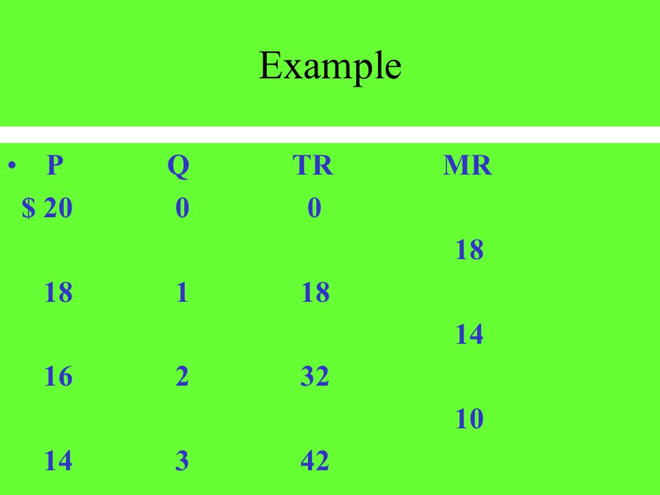
Example P Q TR MR $ 18 14 10

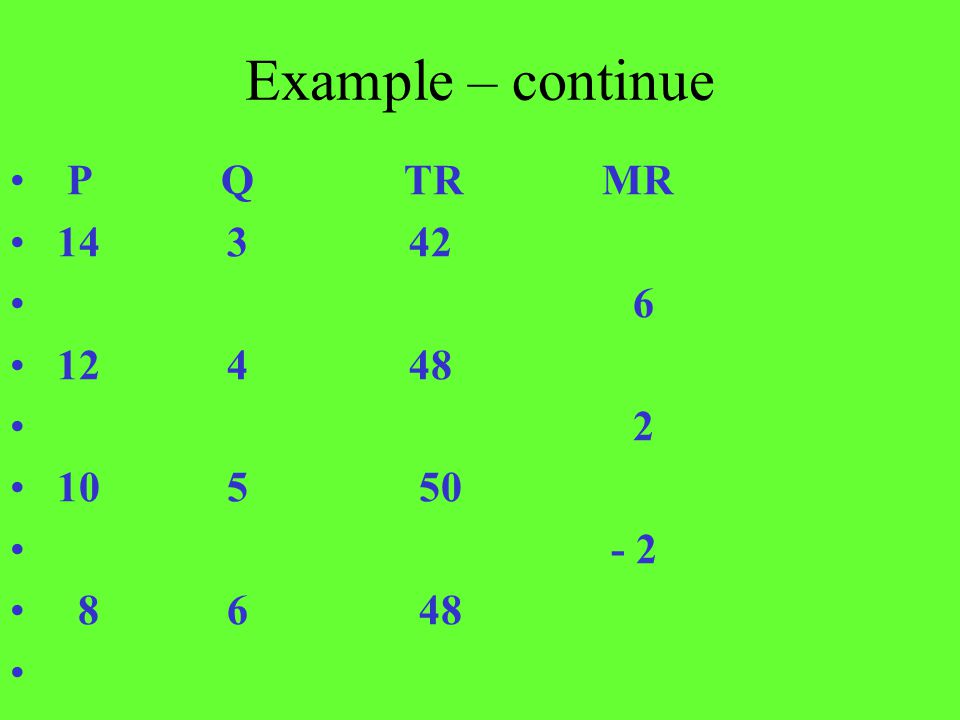
Example – continue P Q TR MR 6 2 - 2

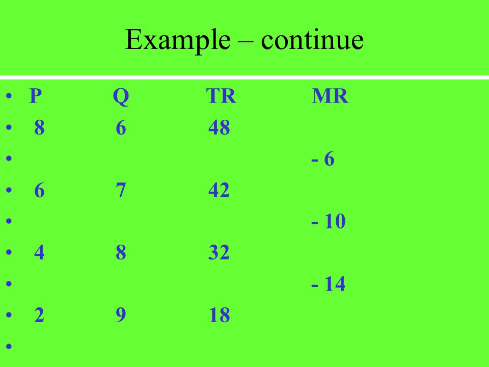
Example – continue P Q TR MR - 6 - 10 - 14

Note MR curve is below the demand curve ,so at each level of output MR < P As output rises, TR rises to a peak the decline . Over the output range where MR > 0 AS P fall , TR rises Over the output range where MR < 0 As P fall , TR fall When MR = 0 , then TR is at its maximum

Short-run Monopoly Equilibrium
A Monopolist in the short-run might have : 1. Positive economic profit , when TR > TC or P > ATC 2. Negative economic profit , when TR < TC or P < ATC 3. Zero economic profit , when TR = TC or P = ATC

Short-run Monopoly Equilibrium
To determine the output level and the price that maximize a monopolist profit, we need to study the behavior of both revenue and cost as output varies .

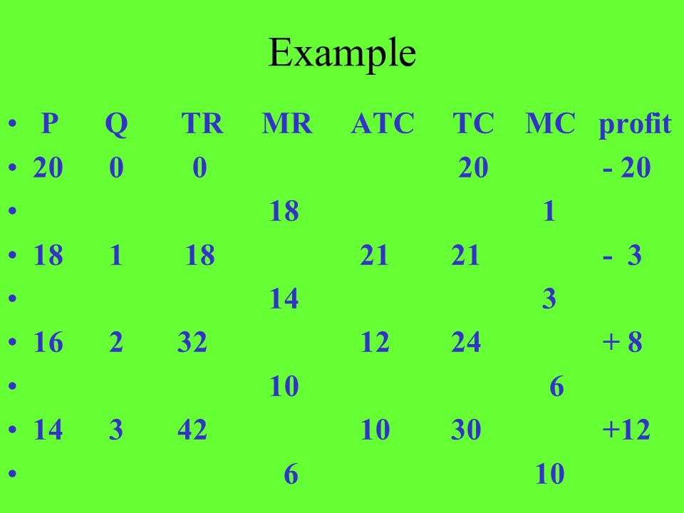
Example P Q TR MR ATC TC MC profit 20 0 0 20 - 20 18 1

Example – Continue P Q TR MR ATC TC MC profit 14 3 42 10 30 12 6 10
Q = 9 units because at that level of output MR = MC = 8 And the equilibrium price is $ 14

Long-run Equilibrium in a Monopoly Market
1. In a monopoly market, profit provide an incentive for new firms to enter . 2. If new firms enter the industry, the equilibrium position will change and the firm will no longer be a monopolist . Therefore, for a monopolist to persist in the long-run , there must be some barriers preventing the new firms from entering ( either Natural or Created barriers ) .

Note A monopolist may make profit even in the long-run , but only if there are natural or created barriers to the entry of new firms .

Cartel as Monopoly Monopoly can arise when :
All firms in an industry agree to cooperate with one another to behave as if they were a single firm . All firms eliminate the competitive behavior among themselves . Such group of firms are called “ Cartel “ .

The Effect of Cartelization
If the industry is cartelized , then 1. profit can be increased 2. output will be reduced 3. price will increase Cartel tend to be unstable because of the incentive for individual firms to violate the output quotas needed to enforce the monopoly.

Note If one firm is cheating, it can increase it profit by increasing its output to the level where MR = MC = P In that case, the firm who is cheating will maximize its profit on the expense of all other firms . But, if all firms are cheating, then price will be pushed back to the competitive level and all firms will be back to zero economic profit where P = ATC and profit = 0

Multi-Price Monopolist
This is the practice of charging some customers higher price than others for identical good or service . Example : Charging children or students lower price than adults .

Perfect Price Discrimination
This occur when a firm charge different price for each unit sold. and charge the customer the maximum price that he is willing to pay for each unit .

Forms of Price Discrimination
1. Discrimination among units of output . 2. Discrimination among buyers .

I. Discrimination among units of output
When the firms charge the same consumer different prices for each unit of output or different prices for each group of output .

II. Discrimination among Buyers
The monopolist charge different prices to different groups of customers on the bases of: Age, education , employment , or other factors . This will work ( increase the profit ) only if each group has different price elasticity of demand for the product . Low price to group with high elasticity . High price to group with low elasticity .

IMPERFECT COMPETITION
CHAPTER 12 IMPERFECT COMPETITION

Imperfect Competition
Can be divided into two types : 1. Imperfect Competition Among Many Firms. This is called “ Monopolistic Competitive Market .” 2. Imperfect Competition Among Few Large Firms . This is called “ Oligopoly Market “

Monopolistic Competition
Is a market structure characterized by a relatively large number of sellers with differentiated products . Each firm attempt to increase its market share by differentiating its product from the output of other firms .

Characteristics of Monopolistic Competitive Market
1. Many firms producing differentiated products, and each product is close substitute for the product produced by other firms . 2. Each firm in the industry make decision based on its own demand and cost conditions . 3. There is freedom of entry into or exit from the industry .

Prediction of the theory
What does this theory of monopolistic competition predicts about the price and the quantity of each firm in the industry? To answer this question, we need to talk about the short-run and the Long-run equilibrium of the firm .

Short-run Equilibrium of the Frim
In the short-run , a firm operating in a monopolistic competitive market is : 1. Similar to a monopoly, so it faces a downward sloping demand curve . 2. It maximize its profit by equating MR with MC ( so MR = MC ) . 3. It may have positive, negative, or Zero economic profit , depending on whether its price greater than, less than, or equal to its ATC .

Long-run Equilibrium of the Firm
1. If the existing firms in short-run are making positive profit, that provide an incentive for new firms to enter the industry. 2.Total demand for the industry product must be shared among larger number of firms. 3. So, each firm get smaller share of total market. This shift the demand curve for each firm to the left and that lower the price . 4. Each monopolistic firm in long-run must have zero economic profit where P = ATC

Excess Capacity Theorem
Excess capacity means : Each firm in a monopolistic competitive market is producing an output less than that corresponding to the lowest point on its ATC curve . Therefore, in monopolistic competitive market, the output produced at a point where ATC is falling , while in perfect competitive market , firms produce their output at lowest possible cost.

Continue Excess capacity = Output produced – Output
Of monopolistic by Perfect produced by Competitive competitive monopolistic firm firm competitive firm Therefore : Excess capacity = Q c Q mc

II. Competition Among Few Firms (Oligopoly )
Is an industry that contains two or more firms , at least one of which produces a significant portion of the industry’s total product .

Characteristics of Oligopoly
1. It faces negatively sloped demand curve . 2. It faces a few competitors . 3. Oligopolies are aware if the interdependence among the decision made by the various firms in the industry. 4. Each firm may take its competitors expected reactions into account when deciding on any action. 5. Prices are administered and products are differentiated .

Types of Oligopoly 1. In some industries there are only few firms operating . 2. In some other industries there are many firms but only few firms dominate the market .

Why Bigness ? Why many industries are dominated by few firms ?
There are several factors , some of these are : 1. Natural Factors 2. Created Factors

Natural Factors Bigness can result naturally from Economies of Scale , i.e. Big firms with large scale have an advantage over small firms with small scale as a result of division of labor . So, Big firms will be more efficient by having lower cost .

Created Causes of Bigness
The number of firms in an industry may decrease and the size of the remaining firms rises due to strategic behavior such as : 1. Buying out rivals ( Acquisition ) 2. Merging with rivals ( Mergers ) 3. Driving rivals into Bankruptcy These practices will lead to a few firms dominate the market and increase the size and market share of these firms .

Is Bigness Natural or Created ?
Most observers would agree that bigness result from a mix of both natural and firm-created causes.

Strategic Behavior and the basic Dilemma of Oligopoly
In deciding on strategies, Oligopolies faces a basic dilemma between competing and cooperating .

Cooperative Outcome If the firms in an oligopolistic industry cooperate, they can maximize their joint profits. If they do this, they will reach what is called “ Cooperative Outcome “ which is similar to what a single monopolist would reach .

Non-Cooperative Outcome
An industry outcome that is reached when all firms proceeds by calculating only their own gains without considering the reaction of others is called “ Non-Cooperative Outcome “ .

Game Theory Is used to study decision making in situations in which a number of players compete, each knowing that others will react to their moves and each taking account of others’ expected reactions when making moves . When Game Theory is applied to Oligopoly, then - the players are the firms . - their game is played in the market . - their strategies are their price or output . - payoffs are their profits .

Duopoly This is a case of two – firm Oligopoly .
In this game there are only two strategies for each firm : To produce an output equal to one-half of the monopoly output. To produce output equal to two-third of the monopoly output .

Note If the two firms cooperate with each other, each one will produce one-half of the monopoly output and that will maximize joint profits. But it leaves each firm with an incentive to alter its output. If A and B cooperate and each produce one-half of the monopoly output and receives one-half of the monopoly profit, the outcome is called “ Cooperative Outcome “ .

Note If A and B make their decision Non – Cooperatively , they reach the Non – Cooperative Outcome , where each produces two-third of the monopoly output and each make less profit than it would if the two firms cooperated . The Non-cooperative outcome is called : “ Nash – Equilibrium “ .

Nash Equilibrium If Nash equilibrium is established by any means, no firm has an incentive to depart from it by altering its own behavior except through cooperation with the other firm. So , in Nash equilibrium, each firm’s best strategy is to maintain its present behavior given the present behavior of the other firm .

Cooperation Or Competition
When firms agree to cooperate in order to restrict output and raise prices, their behavior is called “ Collusion “ Collusive Behavior may occur with or without an explicit agreement .

Explicit Collusion When firms have an explicit agreement to restrict output and raise prices to ensure that they all will maintain their joint profit maximization output . Example : the cartel such as OPEC or Association of Coffee producing countries

Overt or Covert Collusion
Where explicit agreement occur, economists speak of Overt or Covert Collusion . Overt Collusion means the agreement is open . Covert Collusion means the agreement is secret .

Tacit Collusion If there is no explicit agreement occur.
Here all firms behave cooperatively without an explicit agreement .

Types of Competitive Behavior
1. Competition for Market Share 2. Covert Cheating 3. Very long-run Competition

Competition for market share
Firms often compete for market –shares through various forms of non-price competition such as : Advertising Variations in the quality of their product

Covert Cheating Covert rather than overt cheating may occur and be more attractive in an industry that has many differentiated products and in which sales are often by contract between buyers and sellers . Example : Secret discounts Rebates This covert cheating allow a firm to increase its sales at the expense of its competitors .

Very Long-run Competition
When Technology & product characteristics change constantly , there may be advantages to behaving competitively . A firm that behaves competitively in very-long run may be able to maintain a larger market share and earn a larger profit than it would if it cooperate with other firms in the industry .

Cooperative or Non-cooperative Outcome
Empirical research by economists suggests that ; The relative strengths of the incentives to cooperate and to compete vary from industry to industry depending on the characteristics of firms , markets , and the products .

Some of the Characteristics that affect the Strength of Cooperation
The tendency toward joint profit maximization is greater for : 1. Samller numbers of sellers . 2. Producers of similar products . 3. Growing market than in contracting market . 4. Industry with dominant firm . 5. When non-price rivarly is absent or limited . 6. When Barriers to entry of new firms are greater .

Economic Efficiency and Public Policy
Chapter 13 Economic Efficiency and Public Policy

In this chapter we will discuss
Economic Efficiency - Productive efficiency - Allocative Efficiency Efficiency and Market Structure - Perfect Competition - Monopoly - Efficiency in other market Structure Allocative Efficiency and Total Surplus Allocative Efficiency and Market Failure

Economic Efficiency This occurs when the cost of producing a given output is as low as possible. Therefore, Economic efficiency requires that resources not to be wasted .

Example of inefficient use of resources
1. If firms do not use the Least-cost method of production . 2. If the cost of producing the last unit is higher for some firms than for others, which means that the industry’s overall cost of producing the output is higher then necessary. 3. If too much of one product and too little of another product are produced . In all of these cases resources are being used inefficiently.

Pareto-efficiency Efficiency in the use of resources is often called “ Pareto Optimality “ or “ Pareto-Efficiency “ in honor of Italian economist ( Vilfredo Pareto )

Productive Efficiency
This requires that the firm produce any given level of output at : 1. the lowest possible cost. 2. to reach the lowest cost , the firm must combine factors of production so that the ratio of marginal products of each pair of factors equal the ratio of their prices , example : MPL = PL MPK PK

Note Any firm that is not being productively efficient is producing at higher cost than is necessary and that will have lower profit . Productive efficiency implies being on rather than inside , the economy’s production possibility curve .

Allocative Efficiency
Resources are said to be allocatively efficient if it is impossible to produce different bundle of goods to make any one person better off without making at least one other person worse off . The allocation of resources is efficient when each product’s price equals its marginal cost of production . That means MC = P for each good

Note If an individual firm or an individual industry is productively efficient, it does not necessarily means that a given firm or industry is also allocatively efficient . Allocative efficiency is a property of the overall economy i.e. When P = MC in all industries simultaneously. If P > MC in an individual industry, we know that the economy is not allocatively efficient.

Note – continue Any point on the production possibility curve is productively efficient . But, not all points on this curve are allocatively efficient. Any point inside the curve is productively inefficient because it is possible to increase the output without using more resources. Allocative efficiency requires that MC = P for each good . Usually , only one point will be allocatively efficient on the curve .

Efficiency and Market Structure
1. Perfect Competition: In the long-run under perfect competition, each firm produces at the lowest point on its long-run average cost curve ( LRATC ) . No one firm could lower its cost by altering its own production . Therefore, every firm in perfect competition is productively efficient .

Perfect Competition - continue
In perfect competition , all firms in an industry face the same price of their product and that they equate marginal cost to that price ( P = MR = MC ) . Therefore, because all firms in the industry have same cost of their last unit, no relocation of production among firms could reduce the total industry cost . Therefore, in perfect competition, the industry as a whole is productively efficient.

Allocative Efficiency in Perfect competition
Since in perfect competition market, firms maximize their profits by equating P = MC Therefore, when the perfect competition is the market structure for the entire economy where price = Marginal cost, the market is allocatively efficient .

II. Monopoly Productive Efficiency:
Monopolists have an incentive to be productively efficient because their profit will be maximized when they adopt the Lowest cost method to produce any given output. However, the monopolist creates allocative inefficiency because the monopolist’s price always exceeds its marginal cost . ( P > MC )

Efficiency in Other Market Structure
Whenever a firm has any power over the market, the firm is called ( Price Maker ) therefore : 1. It faces a negatively sloped demand curve . 2. Its marginal revenue will be less than its price. 3. Its marginal cost also will be less than its price. This inequality between the price and marginal cost implies allocative inefficiency. Therefore, Oligopoly, and Monopolistic competition are also allocatively inefficient just like the Monopoly.

Allocative Efficiency and Total Surplus
Allocative efficiency occurs where the sum of consumer and producer surplus is maximized. The Consumer Surplus is the value of a good minus the price paid for it . Therefore : The Consumer = Maximum price – Actual price Surplus the consumer is paid willing to pay The Consumer Surplus is the area under the demand curve and above the market price .

The Producer Surplus The producer Surplus is the price that producer receives for a product minus the lowest price that he is prepared to accept for selling it. Producer Surplus = Actual price – Lowest price received by that producer the producer is prepared to accept for the The producer surplus is the area product above the supply curve and below the market price .

Note The sum of producer and consumer surplus is maximized only at the perfectly competitive level of output . This is the only level of output that is allocatively efficient . Since the demand curve represent Price. And supply curve represent marginal cost. Therefore : Demand curve tell us the price for each unit demanded , and the supply curve tell us the marginal cost of each unit produced .

Conclusion Therefore a competitive market is allocatively efficient .
At the intersection point between demand and supply curves P = Mc which is the condition for allocative efficiency for the use of resources . Therefore a competitive market is allocatively efficient .

The Allocative inefficiency of Monopoly
1. The monopolist chooses an output below the competitive level . 2. The monopolist chooses price higher than the 3. As result of this, the consumer surplus will diminish and the producer surplus will increase. Thus, the monopoly is allocatively inefficient because it produces less and charge higher price relative to the competitive market.

CHAPTER ONE The Economic Problem.

Similar presentations

Presentation on theme: "CHAPTER ONE The Economic Problem."— Presentation transcript:

Similar presentations

About project

Feedback

Log in

Auth with social network:

CHAPTER ONE The Economic Problem.

Similar presentations

Presentation on theme: "CHAPTER ONE The Economic Problem."— Presentation transcript:

Similar presentations

About project

Feedback