Download presentation
Presentation is loading. Please wait.

1
Operations Management Dr. Ron Tibben-Lembke
Inventory Management Operations Management Dr. Ron Tibben-Lembke

2
Purposes of Inventory Meet anticipated demand
Demand variability Supply variability Decouple production & distribution permits constant production quantities Take advantage of quantity discounts Hedge against price increases Protect against shortages

3
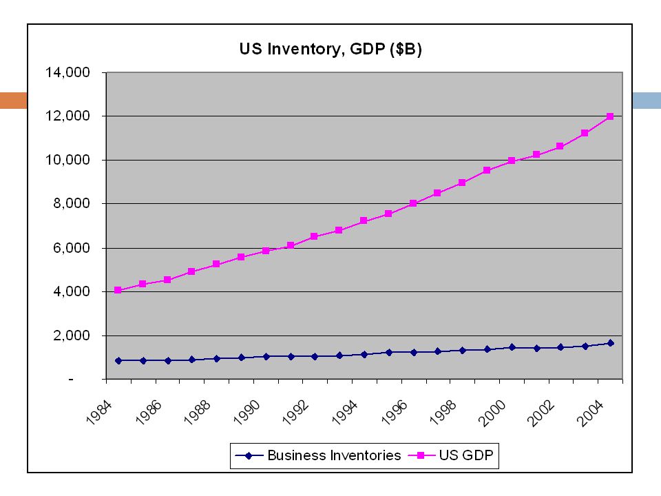
% 2007

5
Source: CSCMP, Bureau of Economic Analysis

6
Two Questions Two main Inventory Questions: How much to buy?
When is it time to buy? Also: Which products to buy? From whom?

7
Types of Inventory Raw Materials Subcomponents Work in progress (WIP)
Finished products Defectives Returns

8
Inventory Costs What costs do we experience because we carry inventory?

9
Inventory Costs Costs associated with inventory: Cost of the products
Cost of ordering Cost of hanging onto it Cost of having too much / disposal Cost of not having enough (shortage)
")
10
Shrinkage Costs How much is stolen? Where does the missing stuff go?
2% for discount, dept. stores, hardware, convenience, sporting goods 3% for toys & hobbies 1.5% for all else Where does the missing stuff go? Employees: 44.5% Shoplifters: 32.7% Administrative / paperwork error: 17.5% Vendor fraud: 5.1%

11
Inventory Holding Costs
Category % of Value Housing (building) cost 4% Material handling 3% Labor cost 3% Opportunity/investment 9% Pilferage/scrap/obsolescence 2% Total Holding Cost 21%
 cost 4% Material handling 3% Labor cost 3% Opportunity/investment 9% Pilferage/scrap/obsolescence 2% Total Holding Cost 21%")
12
Inventory Models Fixed order quantity models Fixed order period models
How much always same, when changes Economic order quantity Production order quantity Quantity discount Fixed order period models How much changes, when always same

13
Economic Order Quantity
Assumptions Demand rate is known and constant No order lead time Shortages are not allowed Costs: S - setup cost per order H - holding cost per unit time

14
EOQ Inventory Level Q* Decrease Due to Optimal Constant Demand Order
Quantity Decrease Due to Constant Demand Time

15
EOQ Inventory Level Instantaneous Q* Receipt of Optimal Optimal
Order Quantity Instantaneous Receipt of Optimal Order Quantity Time

16
EOQ Inventory Level Q* Optimal Order Quantity Time

17
EOQ w Lead Time Inventory Level Q* Optimal Order Quantity Time

18
EOQ Inventory Level Q* Reorder Point (ROP) Time Lead Time
 Time Lead Time")
19
EOQ Inventory Level Q* Average Inventory Q/2 Reorder Point (ROP) Time
Lead Time

20
Total Costs Average Inventory = Q/2 Annual Holding costs = H * Q/2
# Orders per year = D / Q Annual Ordering Costs = S * D/Q Cost of Goods = D * C Annual Total Costs = Holding + Ordering + CoG

21
How Much to Order? Annual Cost Holding Cost = H * Q/2 Order Quantity

22
How Much to Order? Annual Cost Ordering Cost = S * D/Q Holding Cost
= H * Q/2 Order Quantity

23
How Much to Order? Total Cost = Holding + Ordering Annual Cost
Order Quantity

24
How Much to Order? Total Cost = Holding + Ordering Annual Cost
Optimal Q Order Quantity

25
Optimal Quantity Total Costs =

26
Optimal Quantity Total Costs = Take derivative with respect to Q =

27
Optimal Quantity Total Costs = Take derivative with respect to Q =
Set equal to zero

28
Optimal Quantity Total Costs = Take derivative with respect to Q =
Set equal to zero Solve for Q:

29
Optimal Quantity Total Costs = Take derivative with respect to Q =
Set equal to zero Solve for Q:

30
Optimal Quantity Total Costs = Take derivative with respect to Q =
Set equal to zero Solve for Q:

31
Adding Lead Time Use same order size Order before inventory depleted
R = * L where: = average demand rate (per day) L = lead time (in days) both in same time period (wks, months, etc.) d d
 L = lead time (in days) both in same time period (wks, months, etc.) d. d.")
32
A Question: If the EOQ is based on so many horrible assumptions that are never really true, why is it the most commonly used ordering policy? Profit function is very shallow Even if conditions don’t hold perfectly, profits are close to optimal Estimated parameters will not throw you off very far

33
Quantity Discounts How does this all change if price changes depending on order size? Holding cost as function of cost: H = I * C Explicitly consider price:

34
Discount Example D = 10,000 S = $20 I = 20% Price Quantity EOQ c = 5.00 Q < Q >=

35
Discount Pricing X 633 X 666 X 716 Total Cost Price 1 Price 2 Price 3
,000 Order Size

36
Discount Pricing X 633 X 666 X 716 Total Cost Price 1 Price 2 Price 3
,000 Order Size

37
Discount Example Order 666 at a time: Hold 666/2 * 4.50 * 0.2= $ Order 10,000/666 * 20 = $ Mat’l 10,000*4.50 = $45, , Order 1,000 at a time: Hold 1,000/2 * 3.90 * 0.2= $ Order 10,000/1,000 * 20 = $ Mat’l 10,000*3.90 = $39, ,590.00

38
Discount Model 1. Compute EOQ for next cheapest price
2. Is EOQ feasible? (is EOQ in range?) If EOQ is too small, use lowest possible Q to get price. 3. Compute total cost for this quantity Repeat until EOQ is feasible or too big. Select quantity/price with lowest total cost.
 If EOQ is too small, use lowest possible Q to get price. 3. Compute total cost for this quantity. Repeat until EOQ is feasible or too big. Select quantity/price with lowest total cost.")
39
Inventory Management -- Random Demand

40
Random Demand Don’t know how many we will sell
Sales will differ by period Average always remains the same Standard deviation remains constant

41
Impact of Random Demand
How would our policies change? How would our order quantity change? How would our reorder point change?

42
Mac’s Decision How many papers to buy? Average = 90, st dev = 10
Cost = 0.20, Sales Price = 0.50 Salvage = 0.00 Cost of overestimating Demand, CO CO = = 0.20 Cost of Underestimating Demand, CU CU = = 0.30

43
Optimal Policy G(x) = Probability demand <= x Optimal quantity: Mac: G(x) = 0.3 / ( ) = 0.6 From standard normal table, z = =Normsinv(0.6) = Q* = avg + zs = *10 = = 93
 = Probability demand <= x Optimal quantity: Mac: G(x) = 0.3 / ( ) = 0.6 From standard normal table, z = =Normsinv(0.6) = Q* = avg + zs = *10 = = 93")
44
Optimal Policy If units are discrete, when in doubt, round up
If u units are on hand, order Q - u units Model is called “newsboy problem,” newspaper purchasing decision By time realize sales are good, no time to order more By time realize sales are bad, too late, you’re stuck Similar to the problem of # of Earth Day shirts to make, lbs. of Valentine’s candy to buy, green beer, Christmas trees, toys for Christmas, etc., etc.

45
Random Demand – Fixed Order Quantity
If we want to satisfy all of the demand 95% of the time, how many standard deviations above the mean should the inventory level be?

46
Probabilistic Models Safety stock = x m From statistics, Safety stock
Therefore, z = Safety stock & Safety stock = zsL sL From normal table z.95 = 1.65 Safety stock = zsL= 1.65*10 = 16.5 R = m + Safety Stock = = ≈ 367

47
Random Example What should our reorder point be?
demand over the lead time is 50 units, with standard deviation of 20 want to satisfy all demand 90% of the time (i.e., 90% chance we do not run out) To satisfy 90% of the demand, z = 1.28 Safety stock = zσL= 1.28 * 20 = 25.6 R = = 75.6
 To satisfy 90% of the demand, z = Safety stock = zσL= 1.28 * 20 = R = =")
48
St Dev Over Lead Time What if we only know the average daily demand, and the standard deviation of daily demand? Lead time = 4 days, daily demand = 10, standard deviation = 5, What should our reorder point be, if z = 3?

49
St Dev Over LT If the average each day is 10, and the lead time is 4 days, then the average demand over the lead time must be 40. What is the standard deviation of demand over the lead time? Std. Dev. ≠ 5 * 4

50
St Dev Over Lead Time Standard deviation of demand =

51
Service Level Criteria
Type I: specify probability that you do not run out during the lead time Probability that 100% of customers go home happy Type II: proportion of demands met from stock Percentage that go home happy, on average Fill Rate: easier to observe, is commonly used G(z)= expected value of shortage, given z. Not frequently listed in tables
= expected value of shortage, given z. Not frequently listed in tables.")
52
Two Types of Service Cycle Demand Stock-Outs Sum 1,450 55 Type I: 8 of 10 periods 80% service Type II: 1,395 / 1,450 = 96%

53
Fixed-Time period models

54
Fixed-Time Period Model
Every T periods, we look at inventory on hand and place an order Lead time still is L. Order quantity will be different, depending on demand

55
Fixed-Time Period Model: When to Order?
Inventory Level Target maximum Time Period

56
Fixed-Time Period Model: : When to Order?
Inventory Level Target maximum Time Period Period

57
Fixed-Time Period Model: When to Order?
Inventory Level Target maximum Time Period Period

58
Fixed-Time Period Model: When to Order?
Inventory Level Target maximum Period Time

59
Fixed-Time Period Model: When to Order?
Inventory Level Target maximum Period Time

60
Fixed-Time Period Model: When to Order?
Inventory Level Target maximum Period Time

61
Fixed Order Period Standard deviation of demand over T+L =
T = Review period length (in days) σ = std dev per day Order quantity (12.11) =
 σ = std dev per day. Order quantity (12.11) =")
62
Inventory Recordkeeping
Two ways to order inventory: Keep track of how many delivered, sold Go out and count it every so often If keeping records, still need to double-check Annual physical inventory, or Cycle Counting

63
Cycle Counting Physically counting a sample of total inventory on a regular basis Used often with ABC classification A items counted most often (e.g., daily) Advantages Eliminates annual shut-down for physical inventory count Improves inventory accuracy Allows causes of errors to be identified
 Advantages. Eliminates annual shut-down for physical inventory count. Improves inventory accuracy. Allows causes of errors to be identified.")
64
Fixed-Period Model Answers how much to order
Orders placed at fixed intervals Inventory brought up to target amount Amount ordered varies No continuous inventory count Possibility of stockout between intervals Useful when vendors visit routinely Example: P&G rep. calls every 2 weeks

65
ABC Analysis Divides on-hand inventory into 3 classes
A class, B class, C class Basis is usually annual $ volume $ volume = Annual demand x Unit cost Policies based on ABC analysis Develop class A suppliers more Give tighter physical control of A items Forecast A items more carefully

66
Classifying Items as ABC
% Annual $ Volume Items %$Vol %Items A 80 15 B 15 30 C 5 55 A B C % of Inventory Items

67
ABC Classification Solution

68
ABC Classification Solution

Similar presentations